
.png)
TABLE OF CONTENTS
NVIDIA H100 SXM GPUs On-Demand
Key Takeaways
- NVIDIA’s Dynamic Memory Sparsification (DMS) achieves a 376% increase in decoding throughput, reaching 2,687 tokens per second, by compressing the KV cache by 8x during inference.
- Training-free methods like KnormPress can theoretically reach similar speeds, but our benchmarks show that at 80% compression they fail completely, producing unusable outputs.
- To compress memory this aggressively without losing coherence, models must be retrofitted, trained specifically to reason with sparse memory, as shown by the DMS architecture.
- DMS gains its speed by pre-allocating memory pools, which increases upfront Peak VRAM usage compared to standard models. This trade-off enables the massive throughput improvements seen during inference.
- Testing these memory-heavy compression techniques requires high-bandwidth memory. Hyperstack’s NVIDIA H100 80GB SXM instances provide enough VRAM to handle DMS’s pre-allocation while maximizing parallel processing performance.
We love keeping up to date with the latest techniques, so we decided to put NVIDIA KVPress to the test. Spoiler alert: it provides massive memory savings and faster inference.
As Large Language Models scale to massive context windows, the Key-Value (KV) cache has become the primary bottleneck for inference speed and memory. While libraries like KVPress offer compression techniques to shrink this cache, a critical question remains: Can you really delete 80% of a model's memory without degrading its reasoning capabilities?

In this guide, we conduct a head-to-head benchmark on Hyperstack’s H100 infrastructure. We compare a standard training-free approach (KnormPress) against NVIDIA’s state-of-the-art retrofitted model (DMS) to see which approach gives the highest performance and efficiency for the Qwen 3-8B model under demanding workloads.
Understanding The End-to-End KVPress Workflow
Understanding how kvpress achieves these results without requiring you to retrain your model or change its architecture is key to using it effectively. The library is designed as a wrapper for Hugging Face Transformers. Here is the end-to-end flow of how a "Press" actually works during inference:
-png.png?width=1408&height=768&name=Group%202%20(2)-png.png)
- Hook Registration: When you initialise a press (either through the pipeline or via a context manager), the library registers "forward hooks" on every attention layer of the transformer. Think of these as checkpoints that intercept the data flowing through the network.
- The Prefilling Phase: As the model begins the "prefill" phase (processing your prompt), the standard transformer logic runs. It generates Key and Value matrices for every token in your input. However, immediately after each attention layer calculates these matrices, the KVPress hook intercepts them before they are stored in the cache.
- Importance Scoring: Inside the hook, the compression algorithm (e.g.,
KnormPress) analyses these Key and Value tensors. It assigns an "importance score" to every token. The logic is simple: if a token has a low score, it likely won't be attended to by future tokens, so it's safe to discard. - Cache Pruning: Based on your
compression_ratio, KVPress identifies the lowest-scoring tokens. For example, a 0.8 ratio means the bottom 80% of tokens are identified and removed from the tensors. - In-Place Cache Update: The library updates the
past_key_valuesobject in place. Crucially, the transformer doesn't know this happened, it continues as if it has the full context, but its memory footprint is now significantly smaller. - Optimised Decoding: For all subsequent generated tokens (the decoding phase), the model attends only to this compressed cache. Because the cache is smaller, the GPU reads less data from VRAM at every step, directly boosting throughput and reducing latency.
Compression Techniques: KnormPress vs. DMS
While kvpress offers many different compression algorithms ranging from attention-based like SnapKVPress to dimension pruning like ThinKPress our analysis focuses on two distinct techniques to answer the question: Is training necessary for extreme compression?

To test this, we are using a standard training-free (KnormPress) against NVIDIA state-of-the-art retrofitted model (DMS). Here is how they work under the hood:
1. The Training-Free Approach: KnormPress
KnormPress is an easy-to-use method. It assumes that the size of a key vector shows how important it is in the attention mechanism.
-
The Heuristic: It calculates the L2 norm (magnitude) of every key vector in the cache.
-
The Assumption: Tokens with larger key norms contribute more to the attention score (the "Massive Activation" hypothesis).
-
The Selection: It ranks all tokens by their norm and identifies the bottom percentage (e.g., 80%) as redundant.
-
The Action: These low-norm tokens are physically sliced out of the Key and Value tensors in VRAM.
-
The Result: A significantly smaller memory footprint achieved instantly, with zero modifications to the model weights.
2. The Trained Model: Dynamic Memory Sparsification (DMS)
DMS represents the "retrofitted" approach. Instead of guessing which tokens matter, the model was explicitly trained to manage a sparse memory state.
-
Learned Eviction Policy: Unlike other compression techniques, DMS uses a lightweight, trained module to predict an "eviction probability" for every incoming token based on its hidden state.
-
Hybrid Memory Management: It combines a strict "Sliding Window" (protecting the most recent ~512 tokens) with a learned sparse retention policy for the older context.
-
Paged Block Allocation: To achieve massive throughput, DMS pre-allocates memory blocks (PagedAttention style) and routes important tokens into them, rather than constantly resizing tensors.
-
Sparse Reasoning: The model underwent a "retrofitting" training phase (approx. 1,000 steps), teaching it to reason effectively even when 87.5% of its history is missing.
-
The Result: Extreme 8x compression that preserves reasoning capabilities, albeit with higher initial VRAM allocation due to its memory pooling strategy.
By providing this variety, kvpress allows developers to find the perfect balance of memory savings and generation quality for their specific use case, without needing to modify the underlying model architecture or retrain.
How to Install KVPress on Hyperstack
Now, let's walk through the step-by-step process of installing the necessary modules.
Step 1: Accessing Hyperstack
Click to view Step 1 details
First, you will need an account on Hyperstack.
- Go to the Hyperstack website and log in.
- If you are new, create an account and set up your billing information. Our documentation can guide you through the initial setup.
Step 2: Deploying a New Virtual Machine
Click to view Step 2 details
From the Hyperstack dashboard, we will launch a new GPU-powered VM.
- Initiate Deployment: Look for the "Deploy New Virtual Machine" button on the dashboard and click it.
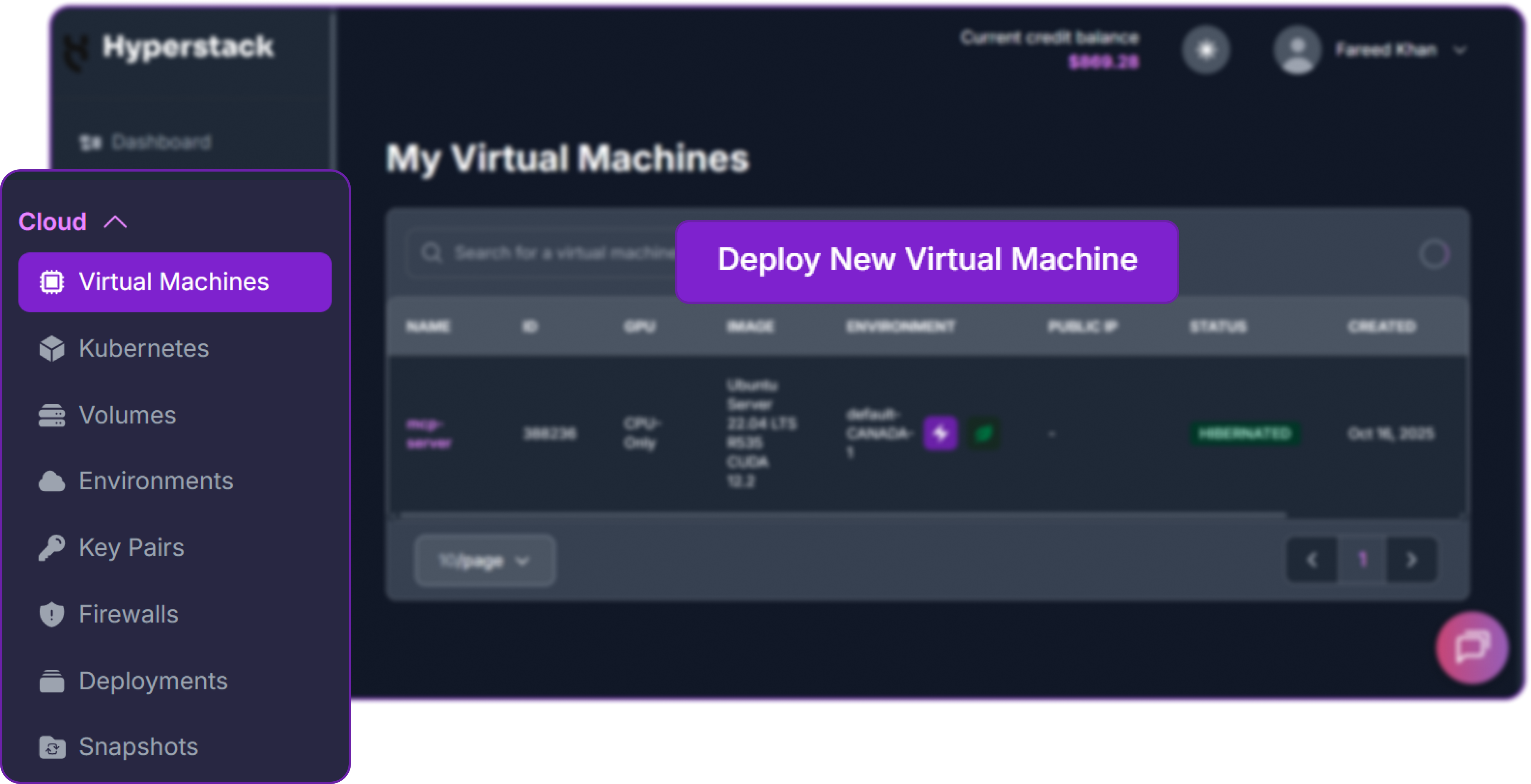
Since we are going to do stress test using the batch processing, it's better to use 1xH100 80GB GPU for our experiments to ensure that we have enough memory to test higher batch sizes and compression ratios without running into out-of-memory errors.

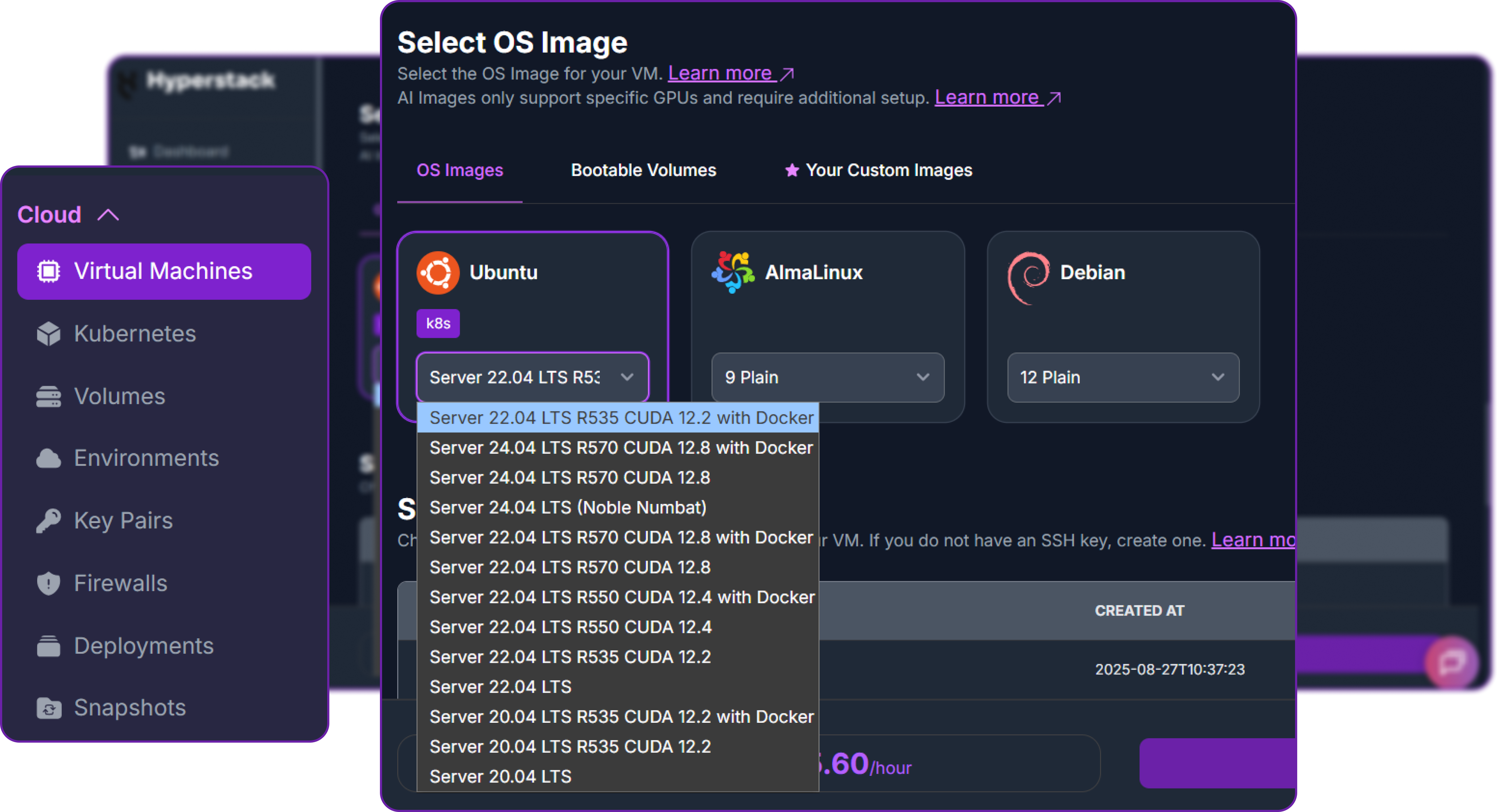
- Choose the Operating System: Select the "Ubuntu Server 22.04 LTS R535 CUDA 12.2 with Docker" image. This provides a ready-to-use environment with all necessary drivers.
- Select a Keypair: Choose an existing SSH keypair from your account to securely access the VM.
- Network Configuration: Ensure you assign a Public IP to your Virtual Machine. This is crucial for remote management and connecting your local development tools.
- Review and Deploy: Double-check your settings and click the "Deploy" button.
Step 3: Accessing Your VM
Click to view Step 3 details
Once your VM is running, you can connect to it.
-
Locate SSH Details: In the Hyperstack dashboard, find your VM details and copy its Public IP address.
-
Connect via SSH: Open a terminal on your local machine and use the following command, replacing the placeholders with your information.
# Connect to your VM using your private key and the VM's public IP
ssh -i [path_to_your_ssh_key] ubuntu@[your_vm_public_ip]
Here you will replace [path_to_your_ssh_key] with the path to your private SSH key file and [your_vm_public_ip] with the actual IP address of your VM.
Once connected, you should see a welcome message indicating you're logged into your Hyperstack VM.
Step 4: Installing KVPress
Click to view Step 4 details
KVPress comes with specific torch.cuda utilities to measure GPU memory usage and time during the prefilling and generation phases of language model inference. It's better to create a virtual environment to avoid dependency conflicts.
So let's create a new environment and install the required libraries:
# Create a new virtual environment (you can name it anything you like)
python3 -m venv kvpress_env
We are naming our environment kvpress_env, but you can choose any name you like. Let's activate the environment:
# Activate the virtual environment
source kvpress_env/bin/activate
We can now install the required libraries using pip:
# Install required libraries
pip install kvpress matplotlib
We are installing kvpress for the KV cache compression and matplotlib for plotting the results. KVpress will automatically handle the installation of its dependencies, including transformers and torch.
Note that we will be using an 8B parameter model for our experiments, if you want to use higher parameter models, you can use flash attention and quantisation techniques to reduce memory usage:
# Install Flash Attention (Highly recommended)
pip install -U flash-attn --no-build-isolation
Once the installation is complete, we can now start coding the benchmarking approach using kvpress .
Benchmarking Extreme Compression: Baseline vs. Knorm vs. DMS
To see how useful trained sparse attention is, we run an experiment on the Qwen 3-8B model with three setups:
- Baseline (0%): The standard dense model with no compression.
- KnormPress (80%): A training-free heuristic that aggressively drops 80% of tokens on the fly.
- DMS (8x): NVIDIA's retrofitted model, specifically trained to manage an 8x compressed cache.
Note: For the DMS configuration, we are using the official pre-trained checkpoints provided by NVIDIA. We did not perform the "retrofitting" training phase ourselves. Instead, we are using NVIDIA open-source weights to evaluate the performance of an already-optimized sparse model.
We can now import the necessary libraries for our performance analysis. This includes libraries for data manipulation, model loading, GPU memory management, and plotting:
# Data manipulation and analysis
import pandas as pd

# Hugging Face utilities for downloading datasets
from huggingface_hub import hf_hub_download

# Progress bar for loops
from tqdm.auto import tqdm

# Serialization and file operations
import pickle
import os

# Warning suppression
import warnings

# Timing utilities
from time import time

# Plotting libraries
import matplotlib.pylab as plt
import matplotlib.ticker as ticker
from matplotlib.colors import LinearSegmentedColormap
import numpy as np

# PyTorch for tensor operations and GPU management
import torch

# Transformers library for LLMs
from transformers import AutoModelForCausalLM, pipeline, AutoTokenizer
from transformers.utils.logging import disable_progress_bar
import transformers
from transformers.cache_utils import DynamicCache

# Garbage collection for memory management
import gc

# KV cache compression library
from kvpress import KnormPress
Most of the libraries are standard for working with language models and GPU performance analysis. KnormPress is the specific compression method we will be using to evaluate the performance of KV cache compression. It basically applies a normalisation technique to the keys and values in the KV cache to reduce memory usage while trying to preserve as much information as possible for generation quality.
Before we start our experiments, we will suppress warnings and disable the progress bar from the transformers library to keep our output clean and focused on the results. This is especially useful when running multiple iterations of model inference, as it prevents cluttering the console with unnecessary logs:
# Suppress warnings for cleaner output
warnings.filterwarnings("ignore")
transformers.logging.set_verbosity_error()
disable_progress_bar()
To properly evaluate the performance of KV cache compression, we need a dataset of prompts that we can feed into the model.
Step 1: Preprocessing Our Eval Dataset
The ShareGPT dataset is a collection of conversations between users and an assistant, which provides a rich source of real-world prompts for our experiments.
It also contains lengthy conversations that allow us to have a high context length, which is important for testing the effectiveness of KV cache compression. We will download the dataset from the Hugging Face Hub, load it into a pandas DataFrame, and extract prompts that are suitable for our performance analysis.
# Download and load the ShareGPT dataset from Hugging Face Hub
DEFAULT_DATASET_URL = "anon8231489123/ShareGPT_Vicuna_unfiltered"

# The dataset file contains conversations between users and the assistant, which we will use to extract prompts for our performance analysis.
DEFAULT_DATASET_FILE = "ShareGPT_V3_unfiltered_cleaned_split.json"

# Download the dataset file and load it into a pandas DataFrame for processing
dataset_path = hf_hub_download(repo_id=DEFAULT_DATASET_URL, filename=DEFAULT_DATASET_FILE, repo_type="dataset")

# Load the dataset into a DataFrame for easier manipulation and filtering
df = pd.read_json(dataset_path)
Once we have the dataset loaded, let's take a look at the structure of the conversations.
# Examine the structure of the conversations in the dataset
sample_conv = df.iloc[0]["conversations"]

# Print the type of the conversation and the first few turns to understand the format of the data
print("Example Conversation Structure:")
print(type(sample_conv))
print("\nFirst 2 turns:")

# Look at the first 2 turns of the conversation to see how the prompts and responses are structured
for turn in sample_conv[:2]:
    print(turn)
This is what we are getting when we print the structure of the conversations:
Example Conversation Structure:
<class 'list'>
First 2 turns:
[
  {
    "from": "human",
    "value": "Summarize the main ideas of Jeff ..."
  },
  {
    "from": "gpt",
    "value": "Here are the main ideas of Jeff Walker's Product ... and improve efficiency."
  }
]
We need to filter the conversations to ensure that we have valid prompts and responses for our performance analysis. We will only keep conversations that have at least 2 messages (a user prompt and an assistant response).
# Filter conversations with at least 2 messages (prompt and completion)
valid_convs = df[df["conversations"].apply(lambda x: len(x) >= 2)]
We will sort the conversations by their ID for reproducibility and then shuffle them with a fixed random seed to ensure that we have a random selection of prompts for our experiments while still being able to reproduce the results in future runs.
# Sort by ID for reproducibility, then shuffle with fixed random seed
sorted_convs = valid_convs.sort_values(by="id")
shuffled_convs = sorted_convs.sample(frac=1, random_state=4387).reset_index(drop=True)
After that we will extract the prompts from the first message of each conversation, ensuring that both the prompt and the completion have at least 10 characters.
# Extract prompts from the first message of each conversation
# Only include conversations where both prompt and completion have at least 10 characters
all_prompts = []

for _, data in shuffled_convs.iterrows():

    prompt = data["conversations"][0]["value"]  # First message is the user prompt
    completion = data["conversations"][1]["value"]  # Second message is the assistant response

    if len(prompt) >= 10 and len(completion) >= 10:
        all_prompts.append(prompt)

print(f"Prepared {len(all_prompts)} prompts from ShareGPT.")
When running the above code, we should see an output like this:
Prepared 88797 prompts from ShareGPT.
So there are 88K valid prompts that we can use for our performance analysis. This is more than enough for our experiments, especially since we will be testing with batch sizes up to 64.
Although we have a large number of prompts, but it's better to specify the GPU device we want to use for our experiments to ensure that we are utilising the correct hardware for model inference and performance measurements.
# Specify the GPU device to use for model inference
device = "cuda:0"
We also need to define the model checkpoints for our baseline and DMS runs. The baseline will use the standard Qwen3-8B model, while the DMS run will use a specific open-source checkpoint from NVIDIA that has been trained to manage an 8x compressed cache.
# Model checkpoints for baseline and DMS runs
base_ckpt = "Qwen/Qwen3-8B"

# DMS checkpoint from Hugging Face Hub, specifically trained for 8x compression
dms_ckpt = "nvidia/Qwen3-8B-DMS-8x"
Our data preprocessing is now complete, and we have a list of prompts ready for our performance analysis.
Step 2: Create Cache Size Calculation Function
We will be using the Qwen3-8B model for our experiments, which is a language model that is suitable for testing KV cache compression techniques because of the reasoning/thinking nature it has.
The next function we need to build is get_size_of_cache, which calculates the memory size of a KV cache in bytes. Let's do that now.
def get_size_of_cache(cache, seen=None):
    if seen is None:
        seen = set()

    obj_id = id(cache)
    if obj_id in seen:
        return 0
    seen.add(obj_id)

    size = 0

    # CASE 1: Custom DMSCache (Paged Attention style)
    if hasattr(cache, "layers") and len(cache.layers) > 0 and hasattr(cache.layers[0], "key_blocks"):
        for layer in cache.layers:
            # We want the logical size of the compressed tokens, not the giant empty pool.
            if hasattr(layer, "cache_seq_lengths") and layer.cache_seq_lengths is not None:
                used_tokens = layer.cache_seq_lengths.sum().item()
                head_dim = layer.head_dim
                element_size = layer.dtype.itemsize if hasattr(layer, "dtype") else 2

                size += 2 * used_tokens * head_dim * element_size
            else:
                if getattr(layer, "key_blocks", None) is not None:
                    size += layer.key_blocks.element_size() * layer.key_blocks.nelement()
                if getattr(layer, "value_blocks", None) is not None:
                    size += layer.value_blocks.element_size() * layer.value_blocks.nelement()
        return size

    # CASE 2: Standard HF DynamicCache
    elif hasattr(cache, "key_cache") and hasattr(cache, "value_cache"):
        for k in cache.key_cache:
            if k is not None and torch.is_tensor(k):
                size += k.element_size() * k.nelement()
        for v in cache.value_cache:
            if v is not None and torch.is_tensor(v):
                size += v.element_size() * v.nelement()
        return size

    # CASE 3: QuantizedCache or newly structured caches
    elif hasattr(cache, "layers"):
        for layer in cache.layers:
            if hasattr(layer, "keys") and layer.keys is not None:
                size += layer.keys.element_size() * layer.keys.nelement()
            if hasattr(layer, "values") and layer.values is not None:
                size += layer.values.element_size() * layer.values.nelement()
        return size

    # CASE 4: Legacy tuple/list structure
    elif isinstance(cache, (list, tuple)):
        for item in cache:
            if isinstance(item, (list, tuple)):
                for tensor in item:
                    if tensor is not None and torch.is_tensor(tensor):
                        size += tensor.element_size() * tensor.nelement()
            elif item is not None and torch.is_tensor(item):
                size += item.element_size() * item.nelement()
        return size

    return 0
This helper function calculates the memory size of a KV cache in bytes. Here's how it works:
-
The function uses a
seenset to track already-processed objects and avoid double-counting shared references, enabling safe recursive size calculation. -
CASE 1 (DMSCache): For NVIDIA's paged attention-style cache, it extracts the number of retained tokens from
cache_seq_lengths, then multiplies by head dimension and element size (2 bytes for fp16/bf16) to get the precise logical cache size, avoiding over-counting from pre-allocated but unused memory pools. -
CASE 2 (DynamicCache): For Hugging Face's standard dynamic cache, it iterates through
key_cacheandvalue_cachelists, summing the memory of all non-null tensors using PyTorch'selement_size()andnelement()methods. -
CASE 3 (QuantizedCache): For newer cache implementations that organize tensors by layer, it accesses
keysandvaluesattributes within each layer and accumulates their memory footprint. -
CASE 4 (Legacy Format): For older tuple or list-based caches, it goes through all the nested items, finds every tensor, and adds up their sizes in bytes.
-
The function returns 0 if the cache object doesn't match any known structure, ensuring robustness across different Transformers library versions.
When it comes to cache implementations, we need to separate the logic for measuring the prefilling phase (when the model processes the input prompt and builds the KV cache) and the generation phase (when the model produces new tokens autoregressively using the KV cache).
Step 3: Creating Prefill State
This way we can get detailed statistics for both phases, including memory usage and time taken, which will help us understand the trade-offs of different compression ratios in a more granular way.
First, let's implement the function to measure the prefilling phase with batch processing.
def get_prefilling_stats(model_ckpt, prompts_batch, press=None):
    """
    Measure prefilling time and KV cache size for batch processing.

    The prefilling phase is when the model processes the full input
    sequence and builds the KV cache.

    This version supports optional KV compression via a context manager.
    """

    # Clean up GPU memory and reset memory tracking
    gc.collect()
    torch.cuda.empty_cache()
    torch.cuda.reset_peak_memory_stats()

    # Load model configuration
    config = AutoConfig.from_pretrained(model_ckpt, trust_remote_code=True)

    # Load tokenizer
    tokenizer = AutoTokenizer.from_pretrained(base_ckpt)

    # Set padding token ID in config to EOS token
    config.pad_token_id = tokenizer.eos_token_id

    # Prepare model loading arguments
    model_kwargs = {"dtype": "auto", "device_map": "auto", "config": config}

    # Some checkpoints require remote code execution
    if "DMS" in model_ckpt:
        model_kwargs["trust_remote_code"] = True

    # Load the language model
    model = AutoModelForCausalLM.from_pretrained(model_ckpt, **model_kwargs)

    # Set padding token to EOS
    tokenizer.pad_token = tokenizer.eos_token

    # Tokenize batch with padding and truncation
    inputs = tokenizer(
        prompts_batch,
        return_tensors="pt",
        padding=True,
        truncation=True,
        max_length=1024
    ).to(device)

    # Warmup: Run a small forward pass
    with torch.no_grad():
        model(inputs.input_ids[:, :10])

    torch.cuda.synchronize()

    # Apply compression context if provided; otherwise use no-op context
    context_manager = press(model) if press else nullcontext()

    # Main measurement: Process full batch and build KV cache
    with torch.no_grad(), context_manager:
        # Initialize dynamic KV cache
        cache = DynamicCache()

        # Measure prefilling time
        start = time()

        # Forward pass with caching enabled
        outputs = model(
            inputs.input_ids,
            past_key_values=cache,
            use_cache=True
        )

        torch.cuda.synchronize()
        prefill_time = time() - start

        # Retrieve the actual cache returned by the model
        actual_cache = (
            outputs.past_key_values
            if hasattr(outputs, "past_key_values")
            else cache
        )

        # Measure total memory footprint of the KV cache
        cache_size = get_size_of_cache(actual_cache)

    # Cleanup
    del model, tokenizer, inputs, cache, outputs

    # Return statistics (cache size converted from bytes to GB)
    return {
        "Prefilling time": prefill_time,
        "Cache Size": cache_size / 1024**3,
    }
In our prefilling stats function, the logic is as follows:
-
- We start by cleaning up GPU memory and resetting memory tracking to ensure accurate measurements unaffected by previous runs.
- Load the model configuration, tokenizer, and prepare model arguments with appropriate settings like
dtype="auto"anddevice_map="auto". - Tokenize the input batch with padding and truncation to 1024 tokens, then run a warmup forward pass to initialize CUDA kernels without measuring startup overhead.
- Setting up an optional compression context manager. If a
pressis provided, we apply it during the forward pass, otherwise, we use a no-op context manager. - We then execute the main prefilling measurement with caching enabled, measure timing, retrieve the actual KV cache, calculate its memory footprint using
get_size_of_cache, then clean up and return results in GB.
Step 4: Creating Generation State
In a similar way, we need to implement the function to measure the generation phase with batch processing. The generation phase is when the model produces new tokens autoregressively using the KV cache built during prefilling.
def get_generation_stats(model_ckpt, prompts_batch, press=None, max_new_tokens=100):
    """
    Measure generation time and peak memory usage for batched decoding.

    The generation phase includes both prefilling (processing the input prompt)
    and autoregressive decoding of new tokens.

    This function supports optional KV compression via a context manager.
    """

    # Clean up GPU memory and reset memory tracking
    gc.collect()
    torch.cuda.empty_cache()
    torch.cuda.reset_peak_memory_stats()

    # Load model configuration
    config = AutoConfig.from_pretrained(model_ckpt, trust_remote_code=True)

    # Load tokenizer
    tokenizer = AutoTokenizer.from_pretrained(base_ckpt)

    # Set padding token ID in config to EOS token
    config.pad_token_id = tokenizer.eos_token_id

    # Prepare model loading arguments
    model_kwargs = {"dtype": "auto", "device_map": "auto", "config": config}

    # Some checkpoints require remote code execution
    if "DMS" in model_ckpt:
        model_kwargs["trust_remote_code"] = True

    # Load the language model
    model = AutoModelForCausalLM.from_pretrained(model_ckpt, **model_kwargs)

    # Set padding token
    tokenizer.pad_token = tokenizer.eos_token

    # Configure deterministic generation settings
    model.generation_config.pad_token_id = tokenizer.pad_token_id
    model.generation_config.eos_token_id = None
    model.generation_config.do_sample = False

    # Tokenize batch with padding and truncation
    inputs = tokenizer(
        prompts_batch,
        return_tensors="pt",
        padding=True,
        truncation=True,
        max_length=1024
    ).to(device)

    # Apply compression context if provided; otherwise use no-op context
    context_manager = press(model) if press else nullcontext()

    # Main measurement: Generate new tokens autoregressively
    with torch.no_grad(), context_manager:
        # Measure total generation time (includes prefilling + decoding)
        start = time()

        model.generate(
            **inputs,
            max_new_tokens=max_new_tokens,
            generation_config=model.generation_config
        )

        torch.cuda.synchronize()
        total_time = time() - start

    # Record peak GPU memory usage during generation
    peak_memory = torch.cuda.max_memory_allocated()

    # Cleanup
    del model, tokenizer, inputs

    # Return statistics (memory converted from bytes to GB)
    return {
        "Total time": total_time,
        "Peak memory usage": peak_memory / 1024**3,
    }
In our generation stats function, the logic is as follows:
-
- Similar to the prefilling function, we start by cleaning up GPU memory and resetting memory tracking for accurate measurements.
- Load the model configuration and tokenizer, ensuring that the padding token is set correctly for batch processing.
- Prepare model loading arguments with optimal settings and load the model.
- Configure the generation settings to ensure deterministic output and proper handling of padding.
- We tokenize the input batch with padding and truncation, then apply the optional compression context manager during generation.
- Measure the total time taken for generation (which includes both prefilling and decoding) and record the peak GPU memory usage during the process.
- Finally, clean up and return the results in GB for memory usage.
Step 5: Combining Stats Logic
It is not possible to directly compare the prefilling and generation stats because they measure different phases of the inference process. However, we can combine them into a single results dictionary that includes both sets of statistics, so let's create a function to do that.
def combine_stats(prefill, gen, batch_size, max_new_tokens=100):
    """
    Combine prefilling and generation statistics into unified metrics.

    This function derives decoding-only time, computes throughput,
    and aggregates key benchmarking metrics.

    Args:
        prefill: Dictionary returned by get_prefilling_stats
        gen: Dictionary returned by get_generation_stats
        batch_size: Number of sequences processed simultaneously
        max_new_tokens: Number of tokens generated per sequence

    Returns:
        dict: Combined statistics including peak memory usage,
              cache size, time-to-first-token (TTFT), and throughput
    """

    # Compute decoding time by subtracting prefilling time
    # Total generation time = prefilling + autoregressive decoding
    gen_time = gen['Total time'] - prefill['Prefilling time']

    # Compute throughput (tokens per second)
    # Formula: (Batch Size × Tokens Generated) / Decoding Time
    throughput = (
        (batch_size * max_new_tokens) / gen_time
        if gen_time > 0 else 0
    )

    # Return combined benchmarking metrics
    return {
        # Peak GPU memory measured during generation phase
        'Peak memory usage': gen['Peak memory usage'],

        # KV cache size measured during prefilling phase
        'Cache Size': prefill['Cache Size'],

        # Time to first token (equals prefilling time)
        'TTFT': prefill['Prefilling time'],

        # Decoding throughput in tokens per second
        'Throughput': throughput
    }
In our combine_stats function, it takes the prefilling and generation statistics, along with the batch size and number of new tokens generated, to compute additional metrics:
-
- We calculate the decoding time by subtracting the prefilling time from the total generation time, giving us the time spent on autoregressive decoding alone.
- Compute the throughput in tokens per second using the formula: (Batch Size × Tokens Generated) / Decoding Time. We also include a check to prevent division by zero in case the decoding time is extremely short.
- Finally, return a dictionary that includes the peak memory usage, cache size, time to first token (which is the prefilling time), and the computed throughput, providing a comprehensive view of the performance characteristics for each compression ratio and batch size.
Step 6: Running Benchmarking Loop
We can now define the compression_ratios and batch_sizes that we want to evaluate, and then iterate through each batch size to measure the prefilling and generation statistics for each compression ratio along with the baseline and DMS runs.
# Initialize results dictionary
stats = {}

# Focused on a single aggressive compression ratio for this benchmark
compression_ratios = 0.8

# # Currently focused on a single batch size for controlled comparison
batch_sizes = [64]

max_prompts_needed = max(batch_sizes)

if len(all_prompts) < max_prompts_needed:
raise ValueError(f"Need at least {max_prompts_needed} prompts, but only have {len(all_prompts)}")
After defining the compression ratios, batch sizes and our DMS based test, we will iterate through batch size and measure the prefilling and generation statistics.
print("Starting Final Benchmark...")  # Iterate over batch sizes

for batch_size in tqdm(batch_sizes, desc="Batch Sizes"):

    # Select the first `batch_size` prompts for evaluation
    # Assumes all_prompts contains sufficiently many prompts
    prompts = all_prompts[:batch_size]

    # Initialize nested dictionary for this batch size
    stats[batch_size] = {}

    # ----------------------------------------------------------
    # 1. Baseline Run (No Compression)
    # ----------------------------------------------------------
    print(f"Running Baseline for BS={batch_size}...")

    # Measure prefilling statistics
    prefill_base = get_prefilling_stats(base_ckpt, prompts)

    # Measure full generation statistics
    gen_base = get_generation_stats(base_ckpt, prompts)

    # ----------------------------------------------------------
    # 2. Knorm Compression Run (80% retention)
    # ----------------------------------------------------------
    print(f"Running Knorm (80%) for BS={batch_size}...")

    # Apply KnormPress compression with 80% retention ratio
    prefill_knorm = get_prefilling_stats(
        base_ckpt,
        prompts,
        press=KnormPress(compression_ratios)
    )

    gen_knorm = get_generation_stats(
        base_ckpt,
        prompts,
        press=KnormPress(compression_ratios)
    )

    # ----------------------------------------------------------
    # 3. DMS Model Run (8× compression variant)
    # ----------------------------------------------------------
    print(f"Running DMS (8x) for BS={batch_size}...")

    # Evaluate DMS checkpoint without external compression
    prefill_dms = get_prefilling_stats(dms_ckpt, prompts)
    gen_dms = get_generation_stats(dms_ckpt, prompts)

    # ----------------------------------------------------------
    # Combine Results
    # ----------------------------------------------------------
    # Each entry aggregates TTFT, throughput, cache size, and peak memory
    stats[batch_size] = {
        'Baseline (0%)': combine_stats(prefill_base, gen_base, batch_size),
        'Knorm (80%)': combine_stats(prefill_knorm, gen_knorm, batch_size),
        'DMS (8x)': combine_stats(prefill_dms, gen_dms, batch_size)
    }

print("Benchmark Complete.")
This will start the benchmarking process:
Loading ShareGPT data...

Prepared 88797 prompts from ShareGPT.

Starting Final Benchmark...
Batch Sizes:   0%|          | 0/1 [00:00<?, ?it/s]

Running Baseline for BS=64...
Running Knorm (80%) for BS=64...

Running DMS (8x) for BS=64...
Batch Sizes: 100%|██████████| 1/1 [01:17<00:00, 77.45s/it]

Benchmark Complete.
Now that our benchmarking is complete we can now look into the results.
Performance Analysis: Throughput vs. Memory Tradeoffs
Let's print the stats variable to see the results for each batch size and compression ratio:
# printing the stats results
print(stats)
These are our results:
{64: {'Baseline (0%)': {'Peak memory usage': 30.883902072906494,
   'Cache Size': 9.0,
   'TTFT': 3.491295337677002,
   'Throughput': 564.4670750984385},
  'Knorm (80%)': {'Peak memory usage': 23.683218479156494,
   'Cache Size': 1.79296875,
   'TTFT': 3.5725390911102295,
   'Throughput': 1271.0371405858396},
  'DMS (8x)': {'Peak memory usage': 50.46891498565674,
   'Cache Size': 5.957980155944824,
   'TTFT': 8.323242664337158,
   'Throughput': 2687.9628813719537}}}
To better understand our results, let's visualise the key metrics (Peak Memory Usage, Cache Size, Throughput, and Time to First Token) across different compression ratios and batch sizes. This will help us see the trade-offs between memory savings and performance as we apply different levels of compression to the KV cache.
Let's create a function to plot these metrics in a clear and informative way, using a 1x4 grid to show all four metrics side by side for easy comparison.
Click to expand Python code
# --- Plotting Function ---
def plot_bar_comparison(stats, batch_size=64, title_suffix=''):
    """
    Plot bar charts comparing key performance metrics across methods.

    Displays Peak Memory, KV Cache Size, Throughput, and TTFT
    for a given batch size.
    """

    # Use clean whitegrid style for readability
    plt.style.use('seaborn-v0_8-whitegrid')

    # Extract data for selected batch size
    data = stats[batch_size]

    # Labels correspond to benchmark variants (Baseline, Knorm, DMS)
    labels = list(data.keys())

    # Metrics to visualize: (dictionary_key, unit, display_title)
    metrics = [
        ('Peak memory usage', 'GB', 'Peak VRAM'),
        ('Cache Size', 'GB', 'KV Cache Size'),
        ('Throughput', 'tok/s', 'Throughput'),
        ('TTFT', 's', 'Time to 1st Token')
    ]

    # Create 4 side-by-side subplots
    fig, axes = plt.subplots(1, 4, figsize=(24, 6))

    # Fixed color scheme: Baseline (gray), Knorm (green), DMS (red)
    colors = ['#cccccc', '#4daf4a', '#e41a1c']

    # Iterate over metrics and generate bar plots
    for idx, (key, unit, title) in enumerate(metrics):

        ax = axes[idx]

        # Extract metric values in label order
        vals = [data[label][key] for label in labels]

        # Create bar chart
        bars = ax.bar(labels, vals, color=colors, edgecolor='black', alpha=0.8)

        # Annotate bars with exact numeric values
        ax.bar_label(bars, fmt=f'%.2f {unit}', padding=3, fontsize=10)

        # Baseline value used for percentage comparison
        baseline_val = vals[0]

        # Throughput: higher is better → show positive improvement
        if key == 'Throughput':

            imp_knorm = (
                ((vals[1] - baseline_val) / baseline_val) * 100
                if baseline_val > 0 else 0
            )
            imp_dms = (
                ((vals[2] - baseline_val) / baseline_val) * 100
                if baseline_val > 0 else 0
            )

            # Place improvement percentages inside bars
            if vals[1] > 0:
                ax.text(1, vals[1]*0.5, f"+{imp_knorm:.0f}%",
                        ha='center', color='white', fontweight='bold')

            if vals[2] > 0:
                ax.text(2, vals[2]*0.5, f"+{imp_dms:.0f}%",
                        ha='center', color='white', fontweight='bold')

        # Memory metrics: lower is better → show reduction percentage
        elif key != 'TTFT':

            imp_knorm = (
                ((baseline_val - vals[1]) / baseline_val) * 100
                if baseline_val > 0 else 0
            )
            imp_dms = (
                ((baseline_val - vals[2]) / baseline_val) * 100
                if baseline_val > 0 else 0
            )

            if vals[1] > 0:
                ax.text(1, vals[1]*0.5, f"-{imp_knorm:.0f}%",
                        ha='center', color='white', fontweight='bold')

            if vals[2] > 0:
                ax.text(2, vals[2]*0.5, f"-{imp_dms:.0f}%",
                        ha='center', color='white', fontweight='bold')

        # Set subplot title and formatting
        ax.set_title(title, fontsize=14, fontweight='bold')
        ax.set_ylabel(unit)
        ax.grid(axis='y', linestyle='--', alpha=0.7)
        ax.set_ylim(bottom=0)

    # Overall figure title
    plt.suptitle(
        f"Performance Comparison: Batch Size {batch_size}{title_suffix}",
        fontsize=16,
        y=1.02
    )

    plt.show()
In our plotting function, we are doing the following:
-
We set up a 1x4 grid of subplots to display the four key metrics side by side for easy comparison.
-
Using a consistent color scheme to differentiate between the Baseline (gray), Knorm (green), and DMS (red) bars.
-
For each metric, we extract the values for the three methods and create a bar chart.
-
We annotate each bar with its exact value for clarity.
-
For throughput, calculate and display the percentage improvement over the baseline directly on the bars.
-
For memory metrics (Peak VRAM and KV Cache Size), we calculate and display the percentage reduction compared to the baseline.
-
Finally, set titles, labels, and gridlines for better readability and display the overall figure title.
Let's execute the plotting function to visualize our results:
# Execute plotting
plot_bar_comparison(stats)
This will generate a comprehensive visualisation of our benchmarking results:

- Throughput : This is the main metric. By slashing the amount of data the GPU has to pull from memory during decoding, the DMS model achieves an +376% increase in tokens per second compared to the baseline. KnormPress also helps, giving a 34% speedup.
- KV Cache Size: As expected, both methods reduce the size of the context window. Knorm explicitly reduces 80% of the tokens. DMS shows a reduction from 9.00 GB to 5.96 GB (a ~34% drop on these shorter prompts). Why isn't DMS at 1/8th the size? Because DMS is explicitly trained to maintain a strict "sliding window" of the most recent 512 tokens to guarantee contextual accuracy. On shorter prompts, this safety window limits the maximum possible compression ratio, but ensures the model never loses its immediate train of thought.
- Peak VRAM (The DMS Trade-off): Look at the first panel. While Knorm successfully reduces overall VRAM usage by 12%, DMS actually spikes Peak VRAM by 63% (up to 50.47 GB). This is a trade-off. To achieve that +376% decoding speed, the DMS implementation uses PagedAttention techniques, pre-allocating massive, empty memory pools upfront so it can route and evict tokens instantly without expensive tensor-resizing operations.
- Time to First Token (TTFT): In the final panel, you will notice DMS takes roughly 8.29 seconds to process the initial prompt, more than double the baseline. Because DMS has to mathematically score every token, track sliding windows, and execute dynamic discarding via chunked processing, it loses the pure parallel processing speed of a standard dense FlashAttention pass during prefilling.
Is retraining really necessary?
The data proves that both methods are incredibly fast at generating text. But it creates an obvious question: if KnormPress is training-free, lowers VRAM, and boosts our speed... why go through the trouble of using NVIDIA's complex, trained DMS model?
The answer lies in what actually happens to the text when you suddenly delete 80% of an AI's memory. For that we need to perform a qualitative analysis of the generated outputs, comparing the baseline, KnormPress, and DMS outputs side by side to see if there are any differences in coherence, relevance, or factual accuracy.
We are going to take a small sample of 10 prompts from our dataset and generate outputs using all three methods for a direct comparison.
# Take a small sample of 10 prompts
sanity_prompts = all_prompts[:10]
This will allow us to see if the aggressive compression from KnormPress has any noticeable impact on the quality of the generated text compared to the baseline and DMS outputs, which will help us understand if retraining is necessary to maintain output quality at high compression ratios.
Click to expand Python code
def generate_text_samples(model_ckpt, prompts, press=None, max_new_tokens=100):
    """
    Generate and decode text outputs for a batch of prompts.

    This function is intended for qualitative comparison between
    baseline and compressed models.
    """

    # Clean up GPU memory before loading model
    gc.collect()
    torch.cuda.empty_cache()

    # Load model configuration and tokenizer
    config = AutoConfig.from_pretrained(model_ckpt, trust_remote_code=True)
    tokenizer = AutoTokenizer.from_pretrained(base_ckpt)

    # CRITICAL: Left-padding is required for batched autoregressive generation
    tokenizer.padding_side = "left"
    tokenizer.pad_token = tokenizer.eos_token

    # Ensure model config uses correct padding token
    config.pad_token_id = tokenizer.eos_token_id

    # Prepare model loading arguments
    model_kwargs = {"dtype": "auto", "device_map": "auto", "config": config}

    if "DMS" in model_ckpt:
        model_kwargs["trust_remote_code"] = True

    # Load the language model
    model = AutoModelForCausalLM.from_pretrained(model_ckpt, **model_kwargs)

    # Tokenize prompts with padding and truncation
    inputs = tokenizer(
        prompts,
        return_tensors="pt",
        padding=True,
        truncation=True,
        max_length=1024
    ).to(device)

    # Apply compression context if provided
    context_manager = press(model) if press else nullcontext()

    # Generate text autoregressively
    with torch.no_grad(), context_manager:
        outputs = model.generate(
            **inputs,
            max_new_tokens=max_new_tokens,
            pad_token_id=tokenizer.pad_token_id,
            eos_token_id=tokenizer.eos_token_id,
            do_sample=False
        )

    # Slice off prompt tokens
    input_length = inputs.input_ids.shape[1]
    generated_ids = outputs[:, input_length:]

    # Decode generated token IDs to text
    generated_texts = tokenizer.batch_decode(
        generated_ids,
        skip_special_tokens=True
    )

    # Cleanup
    del model, tokenizer, inputs, outputs
    gc.collect()
    torch.cuda.empty_cache()

    return generated_texts
In this function, we are doing the following:
- We load the model and tokenizer, ensuring that the tokenizer is set to left-padding mode, which is crucial for correct attention behaviour during autoregressive generation in a batched setting.
- We tokenize the input prompts with padding and truncation, then apply the optional compression context manager during generation.
- We generate new tokens autoregressively, making sure deterministic output by setting
do_sample=False. - After generation, we slice off the input prompt tokens to isolate only the newly generated text, which we then decode back into human-readable strings.
- Finally, we clean up GPU memory to avoid interference with subsequent runs.
Let's run this function for the baseline, KnormPress, and DMS models to compare their outputs side by side.
# --- Run the Sanity Check ---
print("Generating Baseline texts...")
baseline_texts = generate_text_samples(base_ckpt, sanity_prompts, press=None)

print("Generating Knorm (80%) texts...")
knorm_texts = generate_text_samples(base_ckpt, sanity_prompts, press=KnormPress(0.8))

print("Generating DMS (8x) texts...")
dms_texts = generate_text_samples(dms_ckpt, sanity_prompts, press=None)

# --- Combine into a DataFrame ---
sanity_df = pd.DataFrame({
    "Prompt": sanity_prompts,
    "Baseline_Output": baseline_texts,
    "Knorm_80_Output": knorm_texts,
    "DMS_8x_Output": dms_texts
})

# print the DataFrame to compare outputs
print(sanity_df)
This is what the output looks like:
| Prompt | Baseline_Output | Knorm_80_Output | DMS_8x_Output |
|---|---|---|---|
| To convert the Terraform... | depend on the method... | dependUserCode. ’’ ‘haiesan_realodyn... | depend on the method... |
| Traceback (most recent call... | The error message you're... | 爰录音. ’’ ‘haiesan_realodyn... | The error message you're... |
| Write a pitch for... | The movie should be... | The Quart Equationsto clubhouseGT... | The movie should be... |
| node-js get one mongodb... | In Node.js, to retrieve... | _APBAINED{yd zro 爰录音... | In Node.js, to retrieve... |
| i need 50 blog... | for 2024 Here are... | for.logic)UILayout KamiAEA.EdKHKeyId没收吉UPI... | for 2024 Here are... |
| Sure, here is the... | This, in turn, reduces... | ThisGPC /head ,[edException... | This, in turn, reduces... |
| | Fund Name | Return... | Based on the table... | cycl ýboot. ’’ ‘haiesan_realodyn... | Based on the table... |
| Chapter 2: Creating Belief... | Now, let's move on... | [Whitespace/Empty] | Now, let's move on... |
| I want you to... | or maybe a payment... | or)-(aN Equationsto clubhouseGT... | or maybe a payment... |
| I want to send... | Best regards, [Your Name]... | cycl ýboot. ’’ ‘haiesan_realodyn... | Best regards, [Your Name]... |
Let's understand the outputs:
- Speed Gains from Training-Free Methods: Looking at the performance graphs, KnormPress seems like a big win. It drops 80% of its KV cache and increases throughput by 125%. But the text outputs show that this speed comes at a serious cost to the model’s quality.
- Total Context Collapse at Extreme Ratios: Removing 80% of a model’s memory all at once causes it to fail. The Knorm_80_Output column shows repetitive loops, random Chinese characters (爰录音), and meaningless symbols. The model cannot answer the prompts.
- Consistent Output with Retraining (DMS): Even under an 8x memory compression, NVIDIA’s DMS model produces text almost identical to the dense Baseline. It keeps reasoning and formatting intact.
- Why DMS Works: DMS succeeds where Knorm fails because of the retraining, or "retrofitting," phase. The Qwen 3-8B DMS model went through a brief training process that taught it how to navigate and reason effectively even with a heavily sparsified memory state. Unlike Knorm, which drops tokens on the fly based on a simple heuristic, DMS learned how to use the limited memory intelligently, preserving context and maintaining coherent outputs under extreme compression.
- High-Speed Performance: Because DMS maintains the quality of its outputs, its impressive 376% increase in throughput (reaching 2,687 tokens/sec at batch size 64) is practical for real-world use. By preserving reasoning and coherence even under extreme compression, DMS turns memory compression into a true performance improvement, rather than just an experimental optimization.
- Final Conclusion: Retraining is necessary. Training-free methods like KnormPress work well for light compression (20–40%), but for extreme compression of 80% or more, a trained sparse model like DMS is needed to keep the model’s outputs coherent.
Conclusion
In this guide, we tested how far we can compress KV caches using NVIDIA’s KVPress library on Hyperstack’s H100 infrastructure. The main question was: Can we speed up inference a lot without hurting the model’s intelligence?
Our benchmarks showed a clear trade-off. Training-free methods like KnormPress can boost throughput by 125%, but pushing them to 80% compression causes a complete collapse in reasoning. The outputs become unusable.
On the other hand, NVIDIA’s DMS (Dynamic Memory Sparsification) shows that real compression without lossing accuracy needs a different approach. By retraining the Qwen 3-8B model to work with sparse memory, DMS achieves a 376% increase in throughput and reduces the logical cache by 8x, while keeping outputs nearly as coherent as the dense baseline.
This performance comes with a cost. DMS increases peak VRAM by 63% because of pre-allocated memory pools and doubles the Time-to-First-Token (TTFT) latency. It’s best suited for high-throughput, long-context scenarios where raw speed matters more than initial response time or VRAM limits.
In the end, scaling LLMs is about balancing trade-offs. For moderate optimization (20–40% compression), KVPress heuristics give a safe performance boost. But for extreme, production-grade, only retrofitted models like DMS can maintain coherence and performance.
Exceeding Benchmark Performance: Should This Be Used in Production?
The numbers we have seen are impressive, a 376% increase in decoding throughput is a good performance boost for inference costs. But does this mean every developer should immediately implement 8x KV cache compression in their production environments?
The short answer is: No, not everyone.
Like all extreme optimization techniques, Dynamic Memory Sparsification (DMS) and KVPress come with specific trade-offs. Here is what you need to consider before integrating this into your stack:
General Limitations of the Technique
- The TTFT Penalty: If your application requires instantaneous response times (like real-time voice bots), DMS might not be suitable. As our benchmarks showed, the Time-to-First-Token (TTFT) more than doubled because the model has to mathematically score and sort every token during the prefill phase.
- Peak VRAM Actually Increases: If you are running on consumer GPUs or are severely VRAM-constrained, DMS is not the answer. To achieve lightning-fast decoding, DMS relies on pre-allocated memory pools (PagedAttention). While the logical cache is tiny, the physical VRAM footprint reserved on the GPU spikes significantly.
- The Retrofitting Barrier: To get extreme compression (80%+) without output collapse, you cannot just plug-and-play any open-source model. You must use specifically retrofitted checkpoints (like the NVIDIA DMS weights) or invest the compute to train the DMS eviction policy into your own fine-tuned models.
Limitations of Our Experiment
While our benchmarking on Hyperstack clearly demonstrates the architectural trade-offs between dense, training-free, and retrofitted compression, it is important to acknowledge the boundaries of our test:
- This was a qualitative sanity check, not a detailed test: We relied on a 10-prompt qualitative review to see if the model's reasoning collapsed. We did not run the models through full academic benchmarks (like MATH-500 or GPQA) to measure the exact percentage drop in factual accuracy at 8x compression.
- Narrow hardware/workload scope: We tested a single extreme compression ratio (80%) at a single, heavy batch size (64) on an 8B model. Results will scale differently depending on your specific hardware, smaller batch sizes, or massive 70B+ models.
The Bottom Line: Who Should Use This?
You should use training-free KVPress (Knorm, SnapKV) if: You want a free 10% to 30% performance boost on standard Hugging Face models without changing your weights, and your context windows are moderately sized.
You should invest in DMS if: You are operating at enterprise scale, handling massive parallel batches, processing massive context windows (like RAG over entire books), and care far more about raw decoding throughput (tokens per second) than you do about initial prompt latency. For these heavy-duty workloads, running DMS on high-bandwidth infrastructure like Hyperstack’s H100s will yield a massive return on investment.
FAQ
Does extreme compression affect model accuracy?
It depends entirely on the method. As our sanity check shows, aggressive training-free compression (like KnormPress at 80%) destroys model accuracy, leading to hallucinations and gibberish. However, retrofitted models like DMS are specifically trained to handle sparse memory, allowing them to maintain baseline-level accuracy even at 8x compression ratios.
Why does vLLM show much higher throughput for my model than your baseline?
Our baseline uses Hugging Face Transformers model.generate(), the standard interface KVPress is built around. vLLM is a dedicated production inference engine. The throughput gap between them can be significant even on identical hardware. Here are the key reasons:
- Reduction of CPU Launch Overhead via CUDA Graphs: The Transformers (Hugging Face library) generation loop runs in Python, which can add per-token execution overhead. The vLLM inference engine helps reduce this overhead by using CUDA Graphs during decoding. CUDA Graphs record GPU kernel sequences once and replay them, lowering launch latency and improving decoding speed, though CPU control is not completely removed.
- PagedAttention: Standard inference allocates large contiguous memory blocks per request, leading to significant waste. The original vLLM blog shows that in PagedAttention, memory waste only happens in the last block of a sequence, resulting in near optimal memory usage with under 4% waste meaning far more requests fit in GPU memory simultaneously.
- Kernel-level optimizations: vLLM integrates FlashAttention, which fuses the entire multi-head attention computation into a single CUDA kernel, avoiding the expensive step of materializing the full N×N attention matrix to slow GPU memory. The vLLM v1 release also integrates FlashAttention 3 for further gains on H100s.
- Purpose-built scheduler: vLLM scheduler is designed end-to-end for maximum GPU utilization. As described in the vLLM architecture blog, after each step both new and old requests are considered, so the GPU never idles waiting for a fixed batch to finish. Transformers'
generate()has no equivalent, it is built for research flexibility, not production throughput.
Because KVPress hooks directly into that stack (vLLM integration is not yet available). The ~500 tok/s baseline is realistic for Transformers on an H100.
Why does the DMS model consume more VRAM despite compressing the cache?
This is an architectural trade-off. To reach a 376% throughput increase, DMS uses a PagedAttention-style memory pool. It pre-allocates large VRAM blocks so tokens can be routed and removed very quickly without slow dynamic memory operations. Even though the logical cache is small (1.12 GB), the physical VRAM reserved stays high (50 GB).
When should I use KVPress heuristics vs. DMS?
- Use KVPress (Knorm/SnapKV) for easy optimization on any standard model. It is ideal for moderate compression (20-40%) where you want free speedups without changing your model weights.
- Use DMS for dedicated, high-load production environments where you need maximum possible throughput on long-context tasks and are willing to use a specific, retrofitted model checkpoint.
Can I train my own model with DMS?
Yes. While we used the pre-trained Qwen3-8B-DMS-8x checkpoint, the methodology is open. You can apply the DMS retrofitting process to your own custom LLMs using the training recipes provided in NVIDIA's research, allowing you to create sparse variants of Llama 3, Mistral, or other architectures.
Does this work on consumer GPUs?
While kvpress works on consumer hardware, the DMS architecture is memory-hungry due to its pre-allocation strategy. As seen in our benchmarks, the 8B model spiked to over 50GB of VRAM. For testing DMS specifically, we recommend enterprise-grade GPUs like the NVIDIA A100 or H100 (80GB) available on Hyperstack to avoid Out-Of-Memory (OOM) errors.
Subscribe to Hyperstack!
Enter your email to get updates to your inbox every week

