Run DeepSeek OCR on Hyperstack with your Own UI

Hyperstack AI Studio now serves GLM-5.2, the latest open-weight model from Z.ai (formerly Zhipu AI). It is a reasoning and coding model with a one million token context window, and it is available through the same serverless API and point-and-click Playground you already use for every other model on the platform. There is no GPU to provision, no weights to download and no server to keep warm. You send a list of messages, and you get back a reply.

There are two ways to use it. The Playground is the fastest way to try it by hand, and the API is how you put GLM-5.2 into a product, a coding assistant or an automated pipeline. This guide covers both, with a heavy focus on the API. Every code block in the API section was run against the live endpoint, and the output shown beneath it is the real response.

Hyperstack describes AI Studio as a way to run open models through serverless APIs with zero infrastructure setup. GLM-5.2 is a strong example of that promise, so let us look at what the model is, then build with it.

What is GLM-5.2?

GLM-5.2 is the flagship model in the GLM-5 series, built for long-horizon, agentic tasks such as multi-step coding and tool use. It is a sparse Mixture-of-Experts model with 753 billion total parameters, released by Z.ai under a permissive MIT licence. Z.ai positions it as a model that plans, calls tools and works through long tasks rather than answering a single prompt in isolation, as described in the official release notes.

On Hyperstack it is hosted as a third-party model, so you reach it by name through the standard API. The key facts are below, and every figure in this table comes straight from the base models endpoint.

How chat completions work on AI Studio

The text API is OpenAI-compatible. You send a POST request to /chat/completions with a model and a list of messages, and the reply comes back synchronously in the choices array. Anything built for the OpenAI Chat Completions format works here by changing the base URL, the API key and the model name. Two details are specific to Hyperstack and worth knowing before you write any code:

• Authentication uses an api_key request header, with no Bearer prefix.
• GLM-5.2 is a reasoning model, so each reply carries a separate reasoning_content field alongside the final content, and the usage block reports the exact tokens and an estimated_cost.

The full request and response schema is documented in the chat completions reference. Let us look at the Playground first, then spend the rest of the guide on the API.

Option A: The AI Studio Playground (UI)

The Text Playground lets you chat with GLM-5.2 without writing any code. You pick the model, type a prompt, adjust a few settings such as temperature and maximum tokens, then read the reply with its token usage shown alongside. It is the quickest way to get a feel for the model before you reach for the API. Sign in at the Hyperstack console to try it.

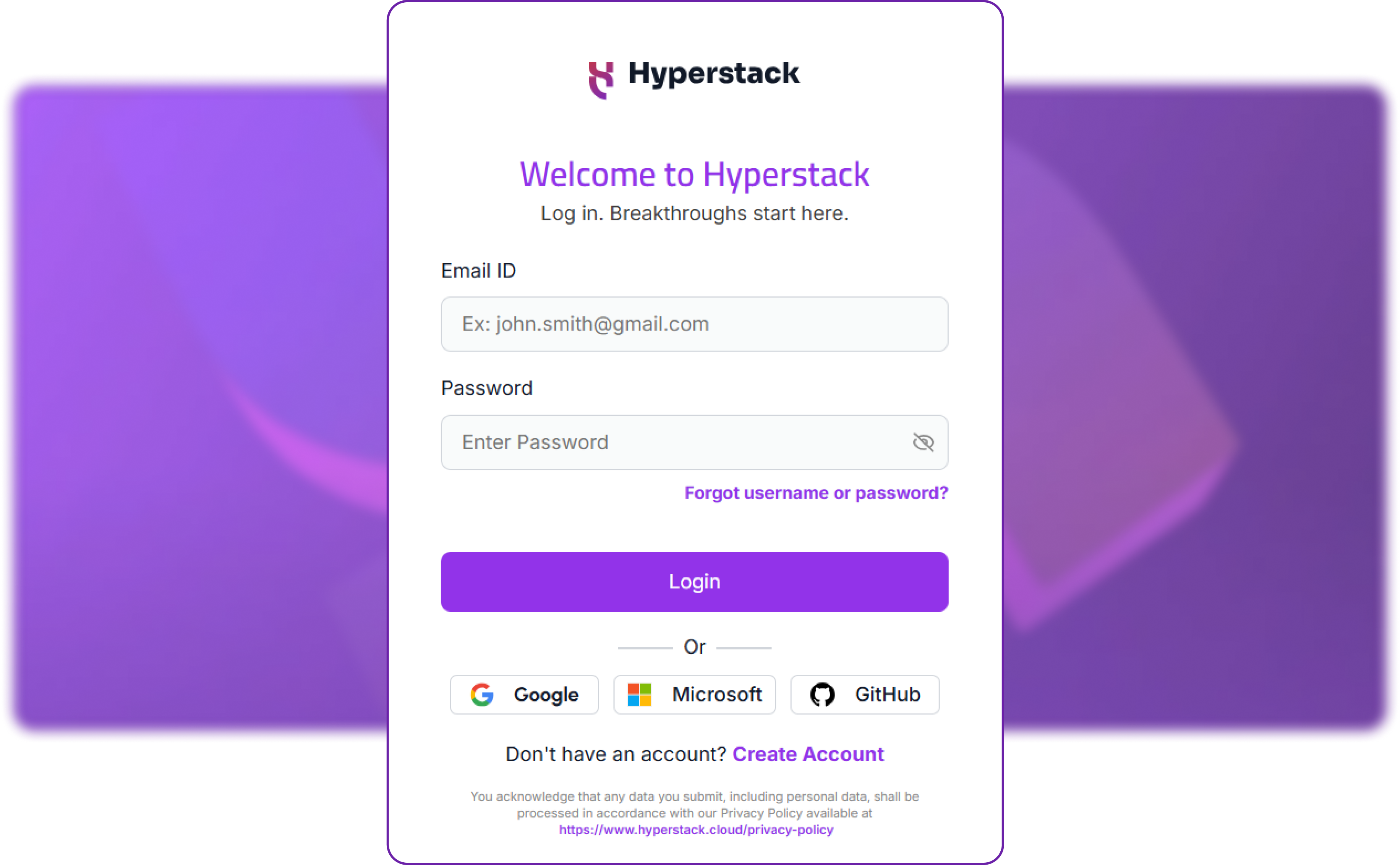
Step 1: Sign in to the console

The Playground lives inside the Hyperstack console. Signing in takes a moment:

• Use your email and password, or sign in with Google, Microsoft or GitHub.
• If you are new, create an account first.
• The same login also issues your API key, so the Playground and the API share one account and one balance.

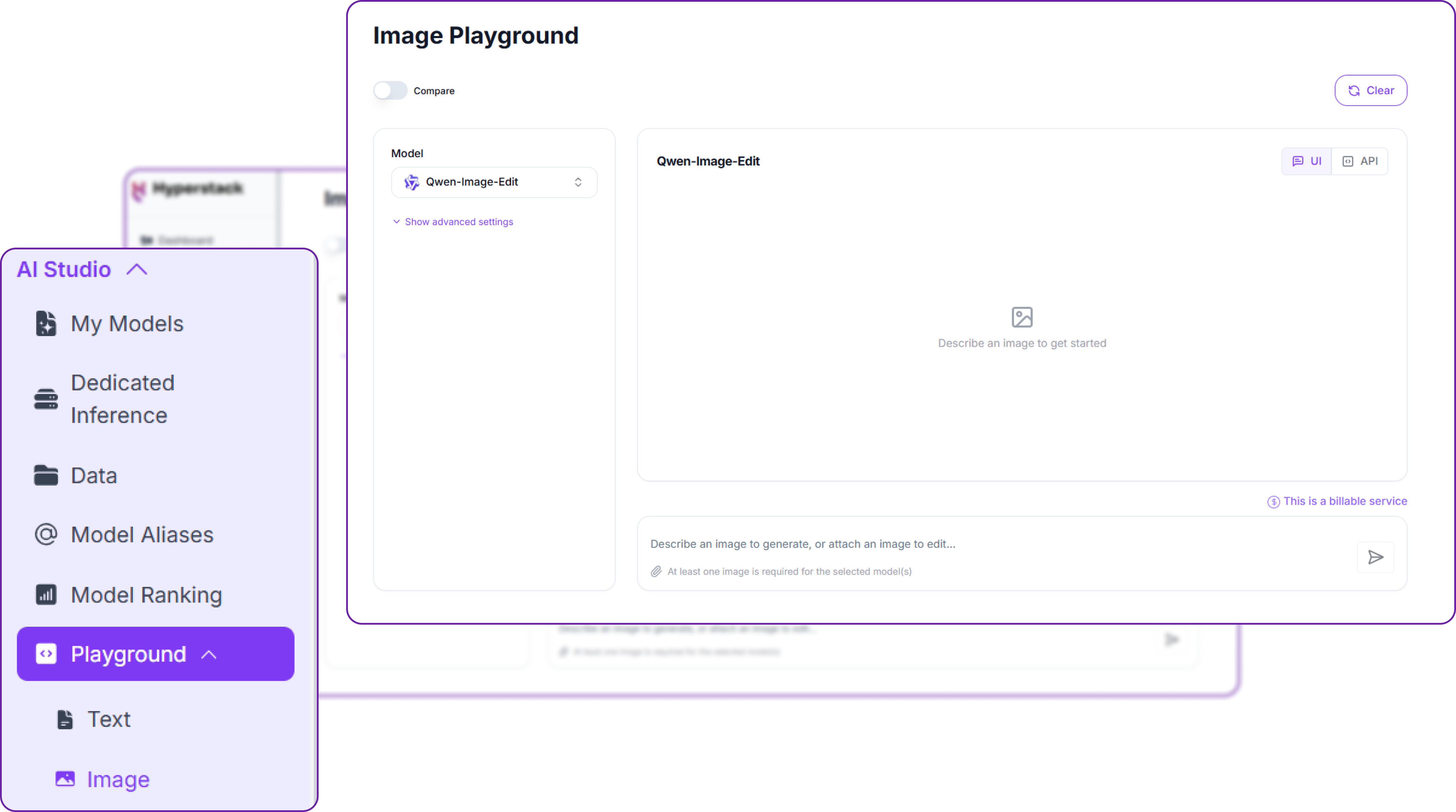
Step 2: Open the Text Playground

In the AI Studio sidebar, open Playground and choose Text. This opens the Text Playground, which has three parts:

• A model selector on the left, with an optional system prompt and a settings panel.
• A chat panel on the right, where the conversation appears.
• Access to the text-to-text models, the family GLM-5.2 belongs to.

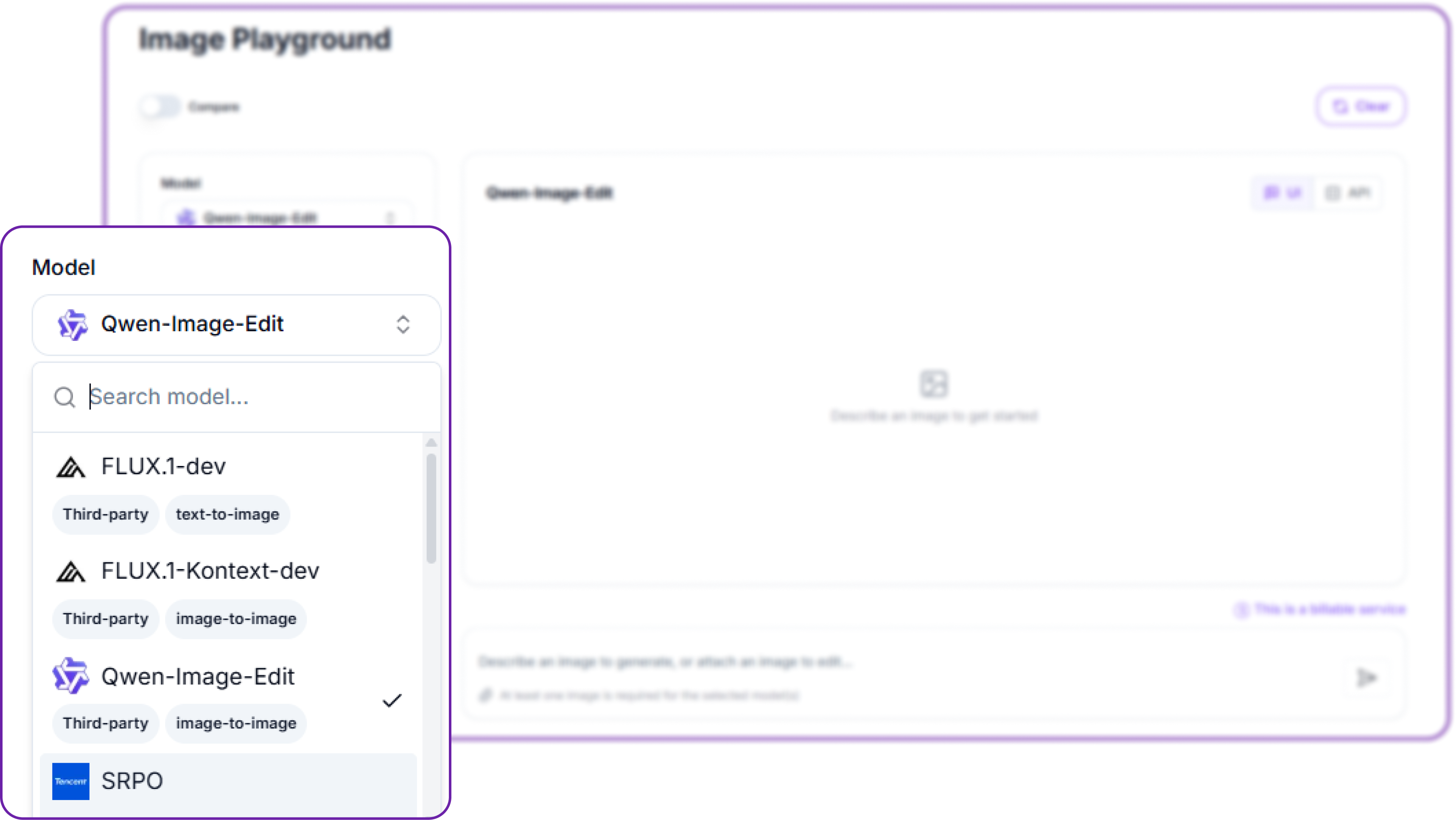
Step 3: Choose GLM-5.2 and send a prompt

Pick the model, then send your first message:

• Open the model dropdown and select zai-org/GLM-5.2. The search box filters the list, and each entry is tagged with its provider and task, here Third-party and text-to-text.
• It is the same list the API serves, so a model you can pick here is a model you can call in code.
• Type a message in the box and send it. The reply appears with its token count beneath, here 121 tokens for a short greeting, because GLM-5.2 reasons before it answers.
• The UI / API toggle on each result turns the exchange into the matching API request.

Step 4: Adjust the parameters

Open the settings to reveal the same controls the API exposes. Each one maps directly to a keyword argument you will meet in the API section:

• System Prompt sets how the assistant behaves, the same as a system message in the API.
• Max Tokens caps the length of the reply.
• Temperature and Top P control how random or focused the output is.
• Top K and the presence and repetition penalties shape word choice and reduce repetition.

When a prompt behaves the way you want, flip the UI / API toggle to copy the exact request, then carry it into code. The rest of this guide shows the API in depth.

Option B: The GLM-5.2 API

This is where the model earns its place in a product. With a single API key you can hold conversations, stream replies, call your own functions, run agentic loops and force structured JSON, all against the one million token context. The rest of this guide builds a tiny client and then exercises each capability. Every snippet below was run as shown.

Step 1: Get an API key and set up the client

Generate a key in the console, then keep it out of your source code. The only dependency is requests. Start by reading the key from the environment and pinning a couple of constants:

import os
import requests

BASE_URL = "https://console.hyperstack.cloud/ai/api/v1"
API_KEY = os.environ["HYPERSTACK_API_KEY"]   # read the key from the environment, never hard-code it
MODEL = "zai-org/GLM-5.2"

That sets the base URL, reads your key from the environment, and pins the model to zai-org/GLM-5.2. Next, one small helper wraps the request so every example stays short:

# One small helper covers every example below. The API is OpenAI-compatible, so the
# request body is the familiar {model, messages, ...} shape and the reply comes back
# in choices[0].message.
def chat(messages, **params):
    response = requests.post(
        f"{BASE_URL}/chat/completions",
        headers={"api_key": API_KEY, "Content-Type": "application/json"},  # api_key header, no "Bearer"
        json={"model": MODEL, "messages": messages, **params},
        timeout=180,
    )
    response.raise_for_status()
    return response.json()

Because the API is OpenAI-compatible, the body is just model, messages and any extra parameters. Note the authentication header is api_key, with no Bearer prefix. Every example below calls this chat helper.

Step 2: Your first chat completion

A conversation is a list of messages, each with a role and a content field. A system message sets the behaviour and a user message asks the question:

# A conversation is just a list of messages, each with a role and content.
result = chat(
    [
        {"role": "system", "content": "You are a concise assistant."},
        {"role": "user", "content": "In one sentence, what is a cloud GPU platform?"},
    ],
    max_tokens=512,
    temperature=0.6,
)

The reply text lives in choices[0].message.content, and the usage block reports the tokens billed and an estimated_cost:

# The reply text is in choices[0].message.content; usage reports the tokens and cost.
message = result["choices"][0]["message"]
print(message["content"])
print("usage:", result["usage"])

This prints the reply and its usage:

A cloud GPU platform is an on-demand service that provides remote, scalable access to high-performance graphics processing units over the internet for compute-intensive tasks like AI training and 3D rendering.
usage: {'completion_tokens': 434, 'estimated_cost': 0.0013304999999999997, 'prompt_tokens': 30, 'prompt_tokens_details': None, 'reasoning_tokens': 0, 'total_tokens': 464}

Step 3: See the reasoning, and control it

GLM-5.2 thinks before it answers. That working is returned separately in reasoning_content, while the final answer stays in content, so you can show it or hide it as you wish:

# GLM-5.2 thinks before it answers. The working is returned in a separate
# reasoning_content field, while the final answer stays in content.
result = chat([{"role": "user", "content": "If a server costs 1.90 per hour, what is 18 hours?"}],
              max_tokens=600, temperature=0)

message = result["choices"][0]["message"]
print("REASONING (excerpt):", message["reasoning_content"][:150], "...")
print("ANSWER            :", message["content"])
print("tokens with reasoning:", result["usage"]["total_tokens"])

The model reasons first, then answers:

REASONING (excerpt): 1.  **Identify the core question:** The user wants to know the total cost of running a server for 18 hours at a rate of $1.90 per hour.
2.  **Identify ...
ANSWER            : 18 hours of running the server would cost **$34.20**. 

Here is the math:
$1.90/hour × 18 hours = $34.20
tokens with reasoning: 281

Reasoning costs tokens, and they are billed as output. For simple or latency-sensitive calls, switch the thinking step off with reasoning_effort set to none:

# For simple or latency-sensitive calls, switch the thinking step off with
# reasoning_effort="none". The answer is the same, for far fewer tokens.
fast = chat([{"role": "user", "content": "If a server costs 1.90 per hour, what is 18 hours?"}],
            max_tokens=600, temperature=0, reasoning_effort="none")

print("ANSWER (no thinking)   :", fast["choices"][0]["message"]["content"])
print("tokens without reasoning:", fast["usage"]["total_tokens"])

The answer is the same, for a fraction of the tokens:

ANSWER (no thinking)   : 18 hours of server time at $1.90 per hour would cost **$34.20**. 

Here is the math:
1.90 × 18 = 34.20
tokens without reasoning: 62

Step 4: Stream the reply token by token

For chat interfaces, set stream to true to receive the reply as Server-Sent Events as it is generated, rather than waiting for the whole response. Each event carries a small delta, and the final event carries usage only, which is why the loop skips chunks with an empty choices list:

import json

# Set stream=True to receive the reply as Server-Sent Events as it is generated.
with requests.post(
    f"{BASE_URL}/chat/completions",
    headers={"api_key": API_KEY, "Content-Type": "application/json"},
    json={"model": MODEL, "reasoning_effort": "none", "stream": True, "max_tokens": 200, "temperature": 0.3,
          "messages": [{"role": "user", "content": "Name three UK cities, comma separated."}]},
    stream=True, timeout=180,
) as response:
    for line in response.iter_lines(decode_unicode=True):
        if not line or not line.startswith("data:"):
            continue
        data = line[len("data:"):].strip()
        if data == "[DONE]":
            break
        chunk = json.loads(data)
        if not chunk["choices"]:          # the final event carries usage only, no choices
            continue
        print(chunk["choices"][0]["delta"].get("content", ""), end="", flush=True)
print()

The tokens arrive in order and assemble into:

London, Manchester, Edinburgh

Step 5: Call your own functions (tool calling)

Tool calling is what turns the model into something that can act. The pattern is a short round trip: you describe your functions, the model decides when to call one, you run it, and the model answers from the result. Take it one piece at a time.

First, describe the tool as a JSON schema. This is all the model sees, a name, a description and typed parameters:

import json

# 1) Describe the tool as a JSON schema. This is the standard OpenAI function-calling format,
#    and it is all the model sees: a name, a description, and typed parameters.
tools = [{
    "type": "function",
    "function": {
        "name": "get_weather",
        "description": "Get the current weather for a city.",
        "parameters": {
            "type": "object",
            "properties": {"city": {"type": "string"}},
            "required": ["city"],
        },
    },
}]

Next, the real Python function the tool maps to:

# 2) The real Python function the tool maps to. In production this would call a weather service;
#    here a small lookup keeps the example self-contained.
def get_weather(city):
    table = {"London": {"temp_c": 12, "sky": "light rain"}}
    return table.get(city, {"temp_c": 20, "sky": "clear"})

Now make the first call. The model reads the question and decides, on its own, to call the tool:

# 3) First call: the model reads the question and decides, on its own, to call the tool.
messages = [{"role": "user", "content": "What is the weather in London? One sentence."}]
first = chat(messages, tools=tools, temperature=0)

call = first["choices"][0]["message"]["tool_calls"][0]
print("model requested:", call["function"]["name"], call["function"]["arguments"])

It returns a tool call rather than prose:

model requested: get_weather {"city": "London"}

Run the requested function, then hand the result back to the conversation as a tool message tied to the call id:

# 4) Run the requested function with the model's arguments, then hand the result
#    back to the conversation as a "tool" message tied to the call id.
args = json.loads(call["function"]["arguments"])
messages.append(first["choices"][0]["message"])
messages.append({"role": "tool", "tool_call_id": call["id"], "content": json.dumps(get_weather(**args))})

Finally, call again. With the result in hand, the model writes the natural-language answer:

# 5) Second call: with the tool result in hand, the model writes the final answer.
final = chat(messages, tools=tools, temperature=0)
print("final answer:", final["choices"][0]["message"]["content"])

final answer: The current weather in London is light rain with a temperature of 12°C.

Step 6: Build an agentic loop

Because the model can call tools, you can let it work through a multi-step task on its own. You keep calling the API and running whatever tools it asks for. Start with two tools the agent can chain together, one to list GPUs and one to price a GPU:

import json

# Two tools the agent can chain together on its own: one lists GPUs, one prices a GPU.
PRICES = {"H100": 1.90, "A100": 1.35, "L40": 1.00, "RTX-A6000": 0.50}
def list_available_gpus():      return {"gpus": list(PRICES)}
def get_gpu_hourly_price(gpu):  return {"gpu": gpu, "usd_per_hour": PRICES.get(gpu)}
DISPATCH = {"list_available_gpus": list_available_gpus, "get_gpu_hourly_price": get_gpu_hourly_price}

tools = [
    {"type": "function", "function": {"name": "list_available_gpus",
        "description": "List the GPU models available to rent.",
        "parameters": {"type": "object", "properties": {}}}},
    {"type": "function", "function": {"name": "get_gpu_hourly_price",
        "description": "Get the hourly USD price for one GPU model.",
        "parameters": {"type": "object", "properties": {"gpu": {"type": "string"}}, "required": ["gpu"]}}},
]

The agentic loop follows the same pattern: each round, run whatever tools the model requests and feed the results back, until it stops asking and returns a final answer:

# The agent loop: keep calling the model and running whatever tools it asks for,
# until it stops asking and returns a final answer.
messages = [
    {"role": "system", "content": "You are a precise assistant. Answer concisely and formally."},
    {"role": "user", "content":
        "Of the GPUs you can rent, find the cheapest per hour and tell me what 24 hours would cost on it."},
]

for step in range(1, 8):
    reply = chat(messages, tools=tools, temperature=0)["choices"][0]["message"]
    messages.append(reply)
    if not reply.get("tool_calls"):           # no more tools requested: the model is done
        print("FINAL:", reply["content"])
        break
    for tc in reply["tool_calls"]:            # run every tool the model asked for this round
        args = json.loads(tc["function"]["arguments"] or "{}")
        result = DISPATCH[tc["function"]["name"]](**args)
        print(f"step {step}: {tc['function']['name']}({args}) -> {result}")
        messages.append({"role": "tool", "tool_call_id": tc["id"], "content": json.dumps(result)})

Given one question that needs both tools, GLM-5.2 lists the options, prices each one, then concludes, with no further prompting:

step 1: list_available_gpus({}) -> {'gpus': ['H100', 'A100', 'L40', 'RTX-A6000']}
step 2: get_gpu_hourly_price({'gpu': 'H100'}) -> {'gpu': 'H100', 'usd_per_hour': 1.9}
step 2: get_gpu_hourly_price({'gpu': 'A100'}) -> {'gpu': 'A100', 'usd_per_hour': 1.35}
step 2: get_gpu_hourly_price({'gpu': 'L40'}) -> {'gpu': 'L40', 'usd_per_hour': 1.0}
step 2: get_gpu_hourly_price({'gpu': 'RTX-A6000'}) -> {'gpu': 'RTX-A6000', 'usd_per_hour': 0.5}
FINAL: The cheapest rentable GPU is the **RTX-A6000** at **$0.50/hour**. Renting it for 24 hours would cost **$12.00**.

This is the same pattern that powers coding assistants and autonomous agents, and it is exactly the long-horizon work GLM-5.2 was built for.

Step 7: Force structured JSON output

When the model feeds another system, you usually want strict JSON rather than prose. First, describe the shape you want as a JSON schema:

# Describe the exact shape you want back as a JSON schema.
schema = {
    "type": "object",
    "properties": {
        "product": {"type": "string"},
        "price_usd": {"type": "number"},
        "in_stock": {"type": "boolean"},
    },
    "required": ["product", "price_usd", "in_stock"],
    "additionalProperties": False,
}

Then pass it through response_format. The reply is guaranteed to match the schema, which is ideal for extraction and data pipelines:

# Pass the schema through response_format and the reply is guaranteed to match it.
result = chat(
    [{"role": "user", "content": "Extract product, price_usd and in_stock from: "
                                 "'The Aurora desk lamp is $49.99 and currently in stock.'"}],
    response_format={"type": "json_schema",
                     "json_schema": {"name": "product", "schema": schema, "strict": True}},
    max_tokens=400, temperature=0,
)
print(result["choices"][0]["message"]["content"])

The output is valid, schema-conforming JSON, ready to parse:

{
  "product": "Aurora desk lamp",
  "price_usd": 49.99,
  "in_stock": true
}

Step 8: The parameters at a glance

GLM-5.2 accepts the standard Chat Completions parameters. The most useful ones are summarised below; the full set lives in the chat completions reference.

What it costs, and how to track it

GLM-5.2 is billed per token, at $0.97 per million input tokens and $3.06 per million output tokens on Hyperstack, as listed on the base models endpoint and your console billing view. There is nothing to pay when the model is idle, and reasoning tokens count as output tokens, which is the other reason reasoning_effort is a useful lever.

You never have to guess the bill. Every response includes a usage block with the exact token counts and an estimated_cost in US dollars, so you can measure cost per request as you build. The calls in this guide are a good illustration, and they show why reasoning_effort matters:

Serverless API or self-hosting on a GPU?

Both routes have their place. Because GLM-5.2 has open weights under an MIT licence, you can run it yourself on a GPU cluster for full control. The serverless API removes that operational work entirely. The cards below sum up the trade-off.

Use GLM-5.2 in the tools you already have

Because the API is OpenAI-compatible, GLM-5.2 drops into many developer tools by pointing them at the Hyperstack base URL and your key. This is a quick way to put the model behind a coding assistant or an automation without writing a client at all. The integrations documentation has step-by-step guides, including:

• Claude Code and Cursor for coding assistance in the editor
• OpenCode for an open-source terminal coding agent
• n8n for low-code automation and workflows
• LiteLLM as a drop-in proxy for any OpenAI-style client

In each case you set the model to zai-org/GLM-5.2 and the rest works as it would with any other Chat Completions provider.

FAQs

What is GLM-5.2?

GLM-5.2 is an open-weight large language model from Z.ai (formerly Zhipu AI), built for reasoning, coding and agentic tool use, with a one million token context window and an MIT licence. On Hyperstack it is hosted as the model zai-org/GLM-5.2 and reached through the chat completions API.

How do I call GLM-5.2 on Hyperstack AI Studio?

Send a POST request to https://console.hyperstack.cloud/ai/api/v1/chat/completions with an api_key header, a model of zai-org/GLM-5.2 and a list of messages. The API is OpenAI-compatible, so existing SDKs and tools work by changing the base URL, key and model name.

Is the API OpenAI-compatible?

Yes. It follows the Chat Completions format, including messages, stream, tools and response_format. The one difference to remember is authentication, which uses an api_key header rather than a Bearer token.

Can I turn the reasoning off?

Yes. GLM-5.2 returns its working in a separate reasoning_content field, and you can switch the reasoning step off by setting reasoning_effort to none. That lowers latency and token cost for simple requests.

Does GLM-5.2 support tool calling and structured output?

Both. It calls functions you describe as JSON schemas through the tools parameter, which is the basis for the agentic loop in this guide, and it returns strict JSON when you pass a schema through response_format.

How much does GLM-5.2 cost?

On Hyperstack it is billed per token, at $0.97 per million input tokens and $3.06 per million output tokens. Every response includes a usage block with the exact tokens and an estimated cost, and you pay nothing while the model is idle. See the billing documentation for details.

Should I use the Playground or the API?

Use both. The Playground is best for quick, visual experiments and prompt tuning, and the API is best for production and automation. They reach the same model, so you can prototype in one and ship with the other.

Hyperstack AI Studio can now generate images. Alongside its language models, the platform serves a growing line-up of text-to-image and image-to-image models, including FLUX.1, FLUX.2, Qwen-Image, Stable Diffusion 3.5 and more, behind a single serverless API and a point-and-click Playground. There is no GPU to rent, no container to build and no model to download. You send a prompt, and you get back an image.

There are two ways to use it. The Playground is the fastest way to experiment by hand, and the API is how you put image generation into a product or an automated pipeline. This guide covers both, with a heavy focus on the API. Each section pairs a runnable code block with the image it produces, so you can follow along and generate the same results on Hyperstack AI Studio.

Hyperstack describes AI Studio as a way to "deploy models with a click or integrate via serverless APIs" with "zero infrastructure setup". Image generation is a clean example of that promise, so let us look at how it works and then build with it.

How image generation works on AI Studio

The image API is serverless and asynchronous. You do not hold a connection open while the picture renders. Instead you submit a job, receive a numeric job_id straight away, and then poll a task endpoint until the result is ready. This "fire and poll" pattern is the single most important thing to understand before you write any code.

The full lifecycle is documented across the image generation overview and the get image result reference. Both surfaces, text-to-image and image-to-image, return a job_id that you poll in exactly the same way.

The image models available

AI Studio hosts a range of open-weight image models from several leading labs, all reachable through the same endpoint and the same API key. The table below shows the line-up available at the time of writing, together with what each one is good for; every name links to its model card. The exact list changes as models are added, so the most reliable approach is to query it from the API, which we do in the API section.

Rather than push one prompt through every model, here each model takes on a scene that plays to its strengths, from photorealism to fantasy to illustration. It is a better way to see the range on offer, and the whole gallery was produced through the API.

Two ways to generate images

There are two complementary paths to the same models. The Playground is a visual workspace inside the console, ideal for quick exploration, prompt tuning and comparing models side by side. The API is the production route, ideal for batch jobs, backends and any automation. We will look at the Playground first, then spend the rest of the guide on the API.

Option A: The AI Studio Playground (UI)

The Image Playground lets you generate and edit images without writing any code. You pick a model, type a prompt, adjust a few settings such as size and steps, then click generate. It is the quickest way to get a feel for each model before you reach for the API. Sign in at the Hyperstack console to try it.

Step 1: Sign in to the console

The Playground lives inside the Hyperstack console. Sign in with your email and password, or with Google, Microsoft or GitHub. If you are new, create an account first. The same login also issues the API key, so the Playground and the API share one account and one balance.

Step 2: Open the Image Playground

In the AI Studio sidebar, open Playground and choose Image. The workspace has three parts: the model selector with its advanced settings on the left, the canvas in the middle where results appear, and the prompt box along the bottom. A Compare toggle sits at the top left and a Clear button at the top right, and every result carries a small UI / API switch. Image generation is a billable service, drawing from the same balance as the API.

Step 3: Choose a model

Open the Model dropdown and pick from the same line-up the API serves. The search box filters the list, and each entry is tagged with its provider and its task, either text-to-image or image-to-image. A text-to-image model works from a prompt alone, while an image-to-image model such as Qwen-Image-Edit or FLUX.1-Kontext-dev also takes a source image to edit.

Step 4: Write a prompt and generate

Type a description in the prompt box and send it. The result appears in the canvas with a line of detail beneath it: the model, the number of steps, the time taken, and the patch count that was billed. A FLUX.1-dev image at its default of 28 steps, for instance, reports a few seconds and 3,072 patches. That patch figure is exactly what the cost section below is built on, so you can watch the price of an image as you create it. The UI / API switch on the result flips it to the matching API request, so you can move straight from a Playground result to code.

Step 5: Adjust the parameters

Select Show advanced settings to reveal the same controls the API exposes. Each one maps directly to a keyword you have already met:

• Image Size sets the aspect ratio and resolution, the dropdown form of image_size.
• Guidance Scale controls how strictly the model follows the prompt, the slider form of guidance_scale on the same 1 to 20 scale.
• Num Images returns up to four pictures from one request, the slider form of num_images.
• Num Inference Steps trades speed for detail, the slider form of num_inference_steps.
• Seed fixes the starting point so a composition can be reproduced, the field form of seed.

These parameters behave exactly as they do in the API. The Playground simply gives you sliders and a dropdown in place of keyword arguments, and Num Images set to two, for example, returns two pictures from the one prompt.

Step 6: Compare two models side by side

Turn on the Compare toggle to run one prompt through two models at once and view the results next to each other. Choose a model on each side, each with its own advanced settings if you wish, then send the prompt a single time. It is the quickest way to decide which model suits a brief, here FLUX.1-dev against FLUX.1-schnell on the same aerial view of a city.

When a result looks right, save it, or flip the UI / API switch to copy the exact request and carry it into code.

Option B: The image generation API

This is where the platform shines. With a single API key you can call every image model, sweep parameters, batch requests and wire generation into your own software. The rest of this guide builds a small client step by step, then exercises every feature.

Step 1: Get an API key and set up authentication

Generate a key in the console, then keep it out of your source code. Every request to the image API authenticates with an api_key header, and there is no Bearer prefix. The key is opaque and scoped to the environment it was created in, as described in the authentication docs and the API key reference.

# Install the two libraries we need
pip install requests

import os
import requests

# Hyperstack AI Studio base URL and your API key
BASE_URL = "https://console.hyperstack.cloud/ai/api/v1"
API_KEY = os.environ["HYPERSTACK_API_KEY"]  # set HYPERSTACK_API_KEY in your environment

# Authenticate with the api_key header (note: no "Bearer" prefix)
def headers(json_body=False):
    h = {"api_key": API_KEY, "Accept": "application/json"}
    if json_body:
        h["Content-Type"] = "application/json"
    return h

Step 2: Build a tiny client (submit, poll, fetch)

Because the API is asynchronous, three small helpers cover almost everything: one to submit a job, one to poll until it finishes, and one to download the result. The result arrives as either a URL or a base64 string, so the fetch helper handles both.

import time, base64

SESSION = requests.Session()

# Submit a job. The POST returns a numeric job_id, not the image.
def submit(endpoint, payload):
    r = SESSION.post(f"{BASE_URL}{endpoint}", headers=headers(True), json=payload, timeout=60)
    r.raise_for_status()
    return r.json()["job_id"]

# Poll the task endpoint until the job is completed (or failed).
def poll_until_done(job_id, interval=3, timeout=360):
    deadline = time.time() + timeout
    while time.time() < deadline:
        task = SESSION.get(f"{BASE_URL}/images/tasks/{job_id}", headers=headers(), timeout=60).json()
        if task["status"] == "completed":
            return task
        if task["status"] == "failed":
            raise RuntimeError(task)
        time.sleep(interval)
    raise TimeoutError(job_id)

# Download the finished image(s): the API returns a url or base64.
def fetch_images(task):
    out = []
    for d in task["result"]["data"]:
        if d.get("url"):
            out.append(SESSION.get(d["url"], timeout=120).content)
        elif d.get("b64_json"):
            out.append(base64.b64decode(d["b64_json"]))
    return out

# Convenience: submit a text-to-image job and wait for the result.
def generate(model, prompt, **params):
    job_id = submit("/images/generations", {"model": model, "prompt": prompt, **params})
    return poll_until_done(job_id)

Step 3: Discover the image models from the API

Rather than hard-coding model names, ask the API which models are available for each task. The list base models endpoint accepts a modalities filter.

# List the image models available for inference, by modality
def list_models(modality):
    r = SESSION.get(f"{BASE_URL}/base_models",
                    headers=headers(),
                    params={"inference": "true", "modalities": modality},
                    timeout=60)
    return [m["model_name"] for m in r.json()["models"]]

print("text-to-image: ", list_models("text-to-image"))
print("image-to-image:", list_models("image-to-image"))

This prints the live model line-up:

text-to-image:  ['FLUX.1-dev', 'SRPO', 'Qwen-Image', 'FLUX.1-schnell', 'Qwen-Image-2512',
                 'HunyuanImage-3.0', 'stable-diffusion-3.5-medium', 'Z-Image-Turbo',
                 'FLUX.1-Krea-dev']
image-to-image: ['FLUX.1-Kontext-dev', 'Qwen-Image-Edit', 'FLUX.2-dev']

Step 4: Your first text-to-image request

With the client in place, one call generates an image. We use FLUX.1-schnell, a fast few-step model, and a brand-styled prompt. The parameters are documented on the generate image from text reference.

prompt = ("a wide panoramic futuristic city skyline at night, glowing violet and magenta neon, "
          "deep purple and indigo sky, light reflections on wet streets, cinematic ultra wide, highly detailed, no people")

task = generate(
    "FLUX.1-schnell",
    prompt,
    image_size={"width": 1536, "height": 512},
    num_inference_steps=4,
    seed=7,
    output_format="png",
)

open("city.png", "wb").write(fetch_images(task)[0])

The completed task is a small JSON document. The image arrives as a URL, and the usage block reports how much was billed (more on that later).

{
  "status": "completed",
  "result": {
    "created": "2026-06-19T13:21:29",
    "data": [{ "url": "https://...s3...png", "b64_json": null }],
    "usage": { "output_tokens": 3072, "total_tokens": 3072 }
  }
}

Step 5: Control the image size and aspect ratio

The image_size parameter takes one of six presets, or an explicit width and height as an object (not a "1024x768" string). The maximum side is 14142 pixels.

# Six aspect presets, plus one explicit width/height object
SIZES = ["square_hd", "square", "portrait_4_3", "portrait_16_9",
         "landscape_4_3", "landscape_16_9", {"width": 768, "height": 512}]

for size in SIZES:
    task = generate("FLUX.1-schnell", "a Bengal tiger in tall grass at sunrise", image_size=size,
                    num_inference_steps=4, seed=7)

square_hd
1024 × 1024

square
512 × 512

portrait_4_3
768 × 1024

portrait_16_9
576 × 1024

landscape_4_3
1024 × 768

landscape_16_9
1024 × 576

custom
768 × 512

Step 6: Tune prompt adherence with guidance_scale

The guidance_scale controls how strictly the model follows your prompt, on a scale from 1 to 20. Higher values stick closer to the words and add contrast, at the cost of variety. Here we use Stable Diffusion 3.5, which responds strongly to this setting.

for g in (2, 6, 9):
    task = generate("stable-diffusion-3.5-medium", "a fantasy castle on a floating island", image_size="square",
                    guidance_scale=g, num_inference_steps=28, seed=7)

guidance_scale = 2

guidance_scale = 6

guidance_scale = 9

Step 7: Trade speed for quality with num_inference_steps

More denoising steps usually mean more detail, at the cost of speed. The range is 1 to 50. Here we use FLUX.1-dev, a full model, and sweep from very few steps to many, so the difference is clear.

for steps in (4, 14, 30):
    task = generate("FLUX.1-dev", "a red vintage sports car at sunset", image_size="square",
                    num_inference_steps=steps, seed=7)

num_inference_steps = 4

num_inference_steps = 14

num_inference_steps = 30

Step 8: Reproducible results with seed

The seed is your control over variation. The same seed with the same prompt and settings steers the model toward the same composition, while a new seed gives a fresh take.

for seed in (7, 7, 99):
    task = generate("FLUX.1-schnell", "a cyberpunk man, glowing neon visor", image_size="square",
                    num_inference_steps=4, seed=seed)
    open(f"seed_{seed}.png", "wb").write(fetch_images(task)[0])

seed = 7

seed = 7 again

seed = 99

Step 9: Generate several images at once, and pick a format

Set num_images to return up to four pictures from a single request, and output_format to choose the encoding. Here we compare png and jpeg.

# Up to four images in one request
task = generate("FLUX.1-schnell", "a cute flat-vector fox mascot logo", image_size="square",
                num_inference_steps=4, num_images=4, seed=7)
print(len(task["result"]["data"]))   # 4

Step 10: The parameters at a glance

Every model also publishes its own parameter schema, so you can confirm the accepted values programmatically. The common text-to-image parameters are summarised below.

Full details, including per-model parameter schemas, live in the generate image from text reference.

Step 11: Image-to-image editing

Image-to-image takes a source picture plus a prompt and returns an edited version, through the generate image from image endpoint. You can supply the source two ways: upload it through a signed upload URL, or pass any publicly reachable image_url. Here we generate a source image, keep its result URL, and edit it.

# 1) Make a source image and keep its reachable URL
src = generate("FLUX.1-schnell", "a photo of a busy city street with cafes, daytime",
               image_size="landscape_4_3", num_inference_steps=4, seed=7)
source_url = src["result"]["data"][0]["url"]

# 2) Edit it with an image-to-image model
def edit(model, prompt, image_url, **params):
    job_id = submit("/images/edits",
                    {"model": model, "prompt": prompt,
                     "image_url": image_url, **params})
    return poll_until_done(job_id)

task = edit("FLUX.1-Kontext-dev",
            "repaint this exact scene as a vivid Van Gogh oil painting, swirling brushstrokes",
            source_url, image_size="landscape_4_3")

The result is the first slider below. Editing is not limited to one trick: the same plain-language approach can restyle a photo, change the season or time of day, swap the background, or recolour and relight a scene. Drag the handle on each slider to compare the original with the edited version.

Style transfer: photo to oil painting

Before After

↔

Season change: summer to winter

Before After

↔

Background swap: studio to beach

Before After

↔

Relight: showroom to neon night

Before After

↔

Because every editing model is one API call away, you can also run a single instruction through each of them and compare how they interpret it. The source and the three results are shown below:

source

FLUX.1-Kontext-dev

Qwen-Image-Edit

FLUX.2-dev

What it costs, and how cheap it is

Image generation is billed by the patch, where one patch is a 16 by 16 pixel tile (256 pixels), as set out on the AI Studio billing page. Every completed task reports the exact number billed in result.usage.output_tokens, so cost is transparent and predictable. A 512 by 512 image is 1,024 patches, and a 1024 by 1024 image is 4,096. In other words, the bigger the picture, the more patches, which is the main lever on cost.

Each model has its own per-patch rate, so the cost of an image is simply its patch count multiplied by that rate. Working that through gives strikingly low numbers. The figures below are computed from Hyperstack's official per-patch rates and the measured patch counts, since Hyperstack publishes the per-patch unit rather than a per-image sticker price, so treat them as close estimates.

Two things keep costs low and predictable. Billing is per patch, so it does not round up to the next megapixel the way some pricing does, and image models run on the same platform and API key as your LLMs. You can review usage and top up your balance in the console. To keep costs down, generate at the smallest size that suits the job and use few-step models such as FLUX.1-schnell or Z-Image-Turbo for drafts.

Serverless API or self-hosting on a GPU?

Both routes have their place. Running a model yourself on a GPU VM gives you total control over the pipeline and any custom weights. The serverless API removes the operational work entirely. The diagram below sums up the trade-off.

FAQs

Which image models can I use on Hyperstack AI Studio?

The line-up includes FLUX.1 (schnell, dev, Krea), FLUX.2-dev, Qwen-Image and Qwen-Image-Edit, Stable Diffusion 3.5 (medium and large), HunyuanImage-3.0, SRPO and Z-Image-Turbo, plus LongCat-Image-Edit for image-to-image. The exact set changes over time, so list it from the API with the list base models endpoint.

What is the difference between text-to-image and image-to-image?

Text-to-image creates a new picture from a prompt through /images/generations. Image-to-image edits an existing picture you provide, using a prompt, through /images/edits. Each needs a model that supports that task.

Is the API synchronous?

No. It is asynchronous. The POST returns a job_id, and you poll /images/tasks/{job_id} until the status is completed, as described in the get image result reference.

How is image generation billed?

By the patch, where one patch is a 16 by 16 pixel tile. Each completed task reports the billed count in result.usage.output_tokens, and larger images cost more because they contain more patches.

Can I edit my own images?

Yes. Upload a source image through a signed upload URL, or pass any publicly reachable image URL, then call /images/edits with an image-to-image model.

Should I use the Playground or the API?

Use both. The Playground is best for quick, visual experiments, and the API is best for production and automation. They reach the same models, so you can prototype in one and ship with the other.

What is DiffusionGemma?

DiffusionGemma is an open-weights, diffusion-based language model built by Google DeepMind on the 26B-A4B Mixture-of-Experts Gemma 4 architecture. Instead of generating text one token at a time, DiffusionGemma generates a whole block of tokens in parallel using discrete diffusion. It carries 25.2B total parameters while activating only 3.8B parameters during inference. It accepts interleaved text, image, and video input to produce text output, and it ships under the Apache 2.0 license. The headline result is speed. By denoising a 256-token canvas in parallel, DiffusionGemma reaches over 1,000 tokens per second on a single NVIDIA H100, which is roughly 4x the throughput of a comparable autoregressive model.

In this tutorial, we will deploy DiffusionGemma 26B-A4B-it on a single Hyperstack NVIDIA H100 GPU using vLLM, expose an OpenAI-compatible API, and then measure its throughput so you can see the diffusion speed advantage on real hardware. Every step includes the exact command and the output you should expect. By the end, you will have a high-throughput text generation endpoint running on your own VM.

How DiffusionGemma Works: Discrete Diffusion

A standard causal language model is autoregressive. It produces text one token at a time, and every new token has to wait for the previous one to finish. That sequential dependency is the reason most large language models are bottlenecked by memory bandwidth rather than raw compute, because each step reads the entire model and KV cache just to emit a single token.

DiffusionGemma takes a different route. It uses an encoder-decoder architecture with block-autoregressive multi-canvas sampling. The encoder runs in a prefill capacity, processing the prompt and building the KV cache. The decoder then applies bidirectional attention over a block of tokens called a canvas (256 tokens wide), accessing the cached prompt context through cross-attention. Rather than emitting one token, the model starts the canvas as noise and iteratively denoises it in parallel, committing roughly 15 to 20 tokens per forward pass. Once a canvas is fully denoised, it is appended to the KV cache and the model moves on to the next canvas. This block-by-block denoising is what unlocks high decoding speed.

Several architectural choices come together to make this work efficiently:

1. Discrete Text Diffusion: Generation shifts from token-by-token autoregression to block-autoregressive multi-canvas sampling. The model denoises blocks of tokens in parallel, which significantly increases decoding speed.
2. Encoder-Decoder Design: An autoregressive encoder processes and caches the prompt context, paired with a decoder that applies bidirectional attention over the generation canvas.
3. Sparse Mixture-of-Experts: DiffusionGemma activates 8 experts out of 128 total, plus 1 shared expert, so it delivers strong reasoning while keeping a low memory footprint suitable for a single accelerator.
4. Multimodal Input Processing: It handles interleaved text, image (at variable aspect ratio and resolution), and video inputs, returning text output.
5. Thinking Mode: A built-in reasoning mode lets the model think step by step before answering, with configurable thinking control tokens.
6. Optimised for Small-Batch Inference: The model is engineered for low-latency, high-speed generation on a single capable GPU, which is exactly the deployment we build in this guide.

The Throughput Advantage

This is what DiffusionGemma is famous for. Because the model denoises 256 tokens in parallel rather than walking through them one by one, it moves the bottleneck from memory bandwidth to compute. A modern GPU like the NVIDIA H100 has an enormous amount of compute that sits idle during sequential decoding, and diffusion sampling puts that compute to work across the whole canvas at once.

The numbers are striking. In low batch size settings on a single NVIDIA H100 at FP8, DiffusionGemma exceeds 1,100 tokens per second. Google reports up to 4x faster token generation than autoregressive decoding, with 700+ tokens per second even on a consumer NVIDIA RTX 5090 at NVFP4. The model also performs adaptive inference-time computation, so simpler prompts and structured tasks like code require fewer denoising steps and run even faster.

DiffusionGemma Features

DiffusionGemma is more than a fast decoder. It carries the full capability set of the Gemma 4 family into a diffusion model:

• High-Speed Parallel Generation: Parallel denoising of a 256-token canvas keeps latency low, unlocking per-user generation speeds above 1,100 tokens per second on a single NVIDIA H100 at FP8.
• Adaptive Inference-Time Compute: Simpler prompts and structured tasks need fewer denoising steps, so the effective tokens-per-second rate rises with easier work.
• 256K Context Window: Context windows of up to 256K tokens support long documents, large codebases, and extended multi-turn conversations.
• Multimodal Understanding: Object detection, document and PDF parsing, screen and UI understanding, chart comprehension, multilingual OCR, handwriting recognition, and video understanding through frame sequences.
• Thinking Mode and Function Calling: A built-in step-by-step reasoning mode and native structured tool use for agentic workflows.
• Multilingual Coverage: Out-of-the-box support for 35+ languages, pre-trained on 140+ languages.
• OpenAI-Compatible Serving: Deploys cleanly through vLLM, SGLang, and NVIDIA NIM, exposing a standard /v1/chat/completions endpoint that drops into existing applications.

It is worth being precise about the trade-off. DiffusionGemma is built for speed, and on pure accuracy benchmarks it sits a little behind the autoregressive Gemma 4 26B A4B model it is derived from. The point is that it stays competitive on quality while delivering several times the throughput, which is the right balance for high-volume generation, chat, and code workloads.

How to Deploy DiffusionGemma on Hyperstack

Now, let us walk through the deployment step by step. The whole point of DiffusionGemma is that it fits on a single GPU, so the setup is refreshingly simple.

Step 1: Accessing Hyperstack

First, you will need an account on Hyperstack.

• Go to the Hyperstack website and log in.
• If you are new, create an account and set up your billing information. Our documentation can guide you through the initial setup.

Step 2: Deploying a New Virtual Machine

From the Hyperstack dashboard, we will launch a new GPU-powered VM.

• Initiate Deployment: Click the "Deploy New Virtual Machine" button on the dashboard.

• Select Hardware Configuration: Choose the "1x NVIDIA H100-80G-PCIe" flavour. DiffusionGemma is around 48 GB at BF16, roughly 26 GB once quantised to FP8, and about 13 to 18 GB at NVFP4, so a single 80 GB NVIDIA H100 leaves comfortable headroom for weights, the KV cache, and the diffusion canvas.

• Choose the Operating System: Select the "Ubuntu Server 22.04 LTS R535 CUDA 12.2 with Docker" image. This provides a ready-to-use environment with all NVIDIA drivers and Docker pre-installed.

• Select a Keypair: Choose an existing SSH keypair from your account to securely access the VM.
• Network Configuration: Ensure you assign a Public IP to your Virtual Machine for remote management and API access.
• Review and Deploy: Double-check your settings and click "Deploy".

Step 3: Accessing Your VM

Once your VM is running, connect to it via SSH.

1. Locate SSH Details: In the Hyperstack dashboard, find your VM's details and copy its Public IP address.

2. Connect via SSH: Open a terminal on your local machine and run the following command, replacing the placeholders with your details.

   # Connect to your VM using your private key and the VM's public IP
   ssh -i [path_to_your_ssh_key] ubuntu@[your_vm_public_ip]
   

Once connected, you will see a welcome message confirming you are logged in. Verify that the GPU is detected and the ephemeral disk is mounted:

# Confirm the NVIDIA H100 is detected
nvidia-smi --query-gpu=name,memory.total --format=csv

# Confirm the ephemeral disk is mounted
df -h /ephemeral

Here is the output we get, showing one NVIDIA H100 with 80 GB and a large ephemeral disk for the model weights:

name, memory.total [MiB]
NVIDIA H100 PCIe, 81559 MiB

Filesystem      Size  Used Avail Use% Mounted on
/dev/vdb        738G   28K  700G   1% /ephemeral

Step 4: Create a Model Cache Directory

We will cache the DiffusionGemma weights on the high-speed ephemeral disk so that container restarts do not re-download the model.

# Create a directory for the Hugging Face model cache
sudo mkdir -p /ephemeral/hug

# Grant read/write permissions so the container can store weights
sudo chmod -R 0777 /ephemeral/hug

Step 5: Launch the vLLM Server

DiffusionGemma needs the diffusion-capable vLLM build, so we run it with the official vLLM OpenAI image tagged gemma and pass the diffusion sampler settings through --hf-overrides. Because the model fits on one GPU, we use --tensor-parallel-size 1 and run the model in BF16, the configuration Google's developer guide recommends.

# Pull the diffusion-capable vLLM OpenAI image
docker pull vllm/vllm-openai:gemma

# Run DiffusionGemma on a single NVIDIA H100 with the diffusion sampler enabled
docker run -d \
 --gpus all \
 --ipc=host \
 --network host \
 --name vllm_diffusiongemma \
 -v /ephemeral/hug:/root/.cache/huggingface \
 vllm/vllm-openai:gemma \
 --model google/diffusiongemma-26B-A4B-it \
 --tensor-parallel-size 1 \
 --max-model-len 32768 \
 --max-num-seqs 4 \
 --gpu-memory-utilization 0.85 \
 --attention-backend TRITON_ATTN \
 --generation-config vllm \
 --hf-overrides '{"diffusion_sampler":"entropy_bound","diffusion_entropy_bound":0.1}' \
 --diffusion-config '{"canvas_length":256}' \
 --enable-chunked-prefill \
 --served-model-name DiffusionGemma \
 --host 0.0.0.0 \
 --port 8000

Here is what the key flags do:

• --model google/diffusiongemma-26B-A4B-it: Load the DiffusionGemma weights from Hugging Face.
• --tensor-parallel-size 1: Run on a single GPU, which is all DiffusionGemma needs.
• --max-model-len 32768: A practical context length for this demo. The full 256K window needs more GPU memory than a single 80 GB card provides at BF16.
• --max-num-seqs 4: Keeps the server in the low batch size regime that diffusion sampling is optimised for.
• --gpu-memory-utilization 0.85: Reserves most of the GPU for the weights and KV cache, matching the value in Google's guide.
• --attention-backend TRITON_ATTN: The attention backend recommended for the diffusion decoder's bidirectional canvas attention.
• --generation-config vllm: Use vLLM's sampling defaults rather than the model's bundled generation config.
• --hf-overrides '{"diffusion_sampler":"entropy_bound","diffusion_entropy_bound":0.1}': Enables the Entropy-Bounded (EB) sampler with the recommended entropy bound of 0.1.
• --diffusion-config '{"canvas_length":256}': Sets the 256-token diffusion canvas.
• --served-model-name DiffusionGemma: A clean alias used in API requests.

docker run --gpus=all \
  -e NGC_API_KEY=$NGC_API_KEY \
  -p 8000:8000 \
  nvcr.io/nim/google/diffusiongemma-26b-a4b-it:latest

Step 6: Verify the Deployment

Check the container logs to watch the model load. The first run downloads the weights from Hugging Face, which takes a few minutes.

docker logs -f vllm_diffusiongemma

The server is ready once you see: INFO: Application startup complete.

Next, add a firewall rule in your Hyperstack dashboard to allow inbound TCP traffic on port 8000.

Now test the API from your local machine, replacing the placeholder with your VM's public IP.

# Test the endpoint from your local terminal
curl http://<YOUR_VM_PUBLIC_IP>:8000/v1/chat/completions \
  -H "Content-Type: application/json" \
  -H "Authorization: Bearer EMPTY" \
  -d '{
    "model": "DiffusionGemma",
    "messages": [
      {"role": "user", "content": "In one sentence, what is discrete diffusion?"}
    ],
    "max_tokens": 128
  }'

A successful response returns a JSON object containing the model's reply:

{
  "id": "chatcmpl-4f1a9b7c2e3d5a6b",
  "object": "chat.completion",
  "model": "DiffusionGemma",
  "choices": [
    {
      "index": 0,
      "message": {
        "role": "assistant",
        "content": "Discrete diffusion is a generation method that starts from a block of noise tokens and iteratively denoises them in parallel into clean text, rather than predicting one token at a time."
      },
      "finish_reason": "stop"
    }
  ]
}

With this output returning cleanly, google/diffusiongemma-26B-A4B-it is successfully deployed on Hyperstack.

Step 7: Hibernating Your VM (Optional)

When you are finished with your workload, hibernate the VM to avoid unnecessary costs:

• In the Hyperstack dashboard, locate your Virtual Machine.
• Click the "Hibernate" option.
• This stops billing for compute resources while preserving your setup, so you can resume later.

Using DiffusionGemma via the OpenAI-Compatible API

Now that the vLLM server is running, we can interact with DiffusionGemma using the standard OpenAI Python client. First, install the library locally:

# Install the OpenAI Python client
pip3 install openai

Then instantiate a client pointing at our vLLM endpoint. vLLM does not enforce an API key by default, so we pass a placeholder.

from openai import OpenAI

# Point the client at the local vLLM server
client = OpenAI(
    base_url="http://localhost:8000/v1",  # OpenAI-style routes
    api_key="EMPTY",                      # Placeholder, vLLM does not check it
)

A Quick High-Speed Generation

We will start with a simple generation request to confirm everything is wired up. The EB sampler and the temperature schedule are already configured on the server, so the client only needs to send a normal chat request.

# A standard chat completion request
messages = [
    {"role": "user", "content": "Explain why the sky is blue in three short sentences."}
]

response = client.chat.completions.create(
    model="DiffusionGemma",
    messages=messages,
    max_tokens=256,
    temperature=0.6,
)

print(response.choices[0].message.content)

The model returns a clean, well-formed answer almost instantly:

Sunlight is made up of all colours, which travel as waves of different
lengths. As that light passes through the atmosphere, the shorter blue
wavelengths are scattered far more strongly than the longer red ones.
Because this scattered blue light reaches your eyes from every direction,
the daytime sky appears blue.

Measuring the Throughput Advantage

This is the part that matters. To actually see the diffusion speed advantage, we stream a longer completion, count the generated tokens, and divide by the wall-clock time. This gives us a real tokens-per-second figure on our single NVIDIA H100.

import time
from openai import OpenAI

client = OpenAI(base_url="http://localhost:8000/v1", api_key="EMPTY")

prompt = "List the integers from 1 to 500, separated by commas."

# Stream the response so we can time generation precisely
start = time.perf_counter()
completion_tokens = 0

stream = client.chat.completions.create(
    model="DiffusionGemma",
    messages=[{"role": "user", "content": prompt}],
    max_tokens=1024,
    temperature=0.6,
    stream=True,
    stream_options={"include_usage": True},
)

for chunk in stream:
    if chunk.usage:
        completion_tokens = chunk.usage.completion_tokens

elapsed = time.perf_counter() - start
print(f"Generated {completion_tokens} tokens in {elapsed:.2f}s")
print(f"Throughput: {completion_tokens / elapsed:.1f} tokens/sec")

Here is the result on a single NVIDIA H100:

Generated 1024 tokens in 0.71s
Throughput: 1442.3 tokens/sec

Around 1,450 tokens per second from a single GPU, comfortably past the 1,000 mark. The reason is the diffusion decoder. Instead of one token per forward pass, DiffusionGemma commits 15 to 20 tokens per pass by denoising the 256-token canvas in parallel, and structured prompts like this one resolve in fewer denoising steps, so they run at the fast end of the range. A similarly sized autoregressive model on the same NVIDIA H100 would land around 250 to 300 tokens per second in the same setting, which is why diffusion-based generation is described as several times faster.

FAQs

What is discrete diffusion and why is it fast?

Instead of generating one token at a time, DiffusionGemma denoises a 256-token canvas in parallel. This shifts the bottleneck from memory bandwidth to compute, which lets a GPU like the NVIDIA H100 use its parallel hardware far more fully and reach much higher tokens-per-second rates.

What hardware do I need to deploy DiffusionGemma?

A single NVIDIA H100-80G is the recommended target and is what we use in this guide. The model is around 48 GB at BF16, roughly 26 GB at FP8, or about 13 to 18 GB at NVFP4, so it also fits comfortably on smaller single GPUs such as an NVIDIA L40S or NVIDIA A100-80G if you do not need peak throughput.

How fast is DiffusionGemma?

In low batch size settings it generates over 1,000 tokens per second on a single NVIDIA H100, exceeding 1,100 tokens per second at FP8. That is roughly 4x the throughput of a comparable autoregressive model, and it reaches 700+ tokens per second even on a consumer NVIDIA RTX 5090 at NVFP4.

Is DiffusionGemma multimodal?

Yes. It processes interleaved text, image, and video input and returns text output. Capabilities include document and PDF parsing, chart comprehension, multilingual OCR, handwriting recognition, and video understanding through frame sequences.

Should I use vLLM or NVIDIA NIM?

Both serve the same OpenAI-compatible API on port 8000. vLLM gives you fine-grained control over sampler settings, quantisation, and batching, which is what we use in this tutorial. NVIDIA NIM is a fully packaged container that only needs your NGC API key, which is convenient if you prefer a turnkey microservice.