How to Optimise the KV Cache: A Guide to Faster, Cheaper LLM Inference

Serving LLMs efficiently comes down, again and again, to one component: the KV cache. After the model weights themselves, it is the single biggest consumer of NVIDIA GPU memory during inference, and it is the reason long contexts and large batches get expensive fast.

If you serve LLMs at any scale, optimising the KV cache is the highest-leverage thing you can do. It decides how long a context you can serve, how many users you can batch together, and ultimately your cost per token.

Our latest guide explains what the KV cache is, why it becomes a bottleneck, and the full landscape of techniques to optimise it, from a one-line quantisation flag you can turn on today to the architectural changes powering frontier models. Throughout, we anchor the theory to numbers you can reproduce and code you can run.

Why The KV Cache Exists (And Why It Hurts)

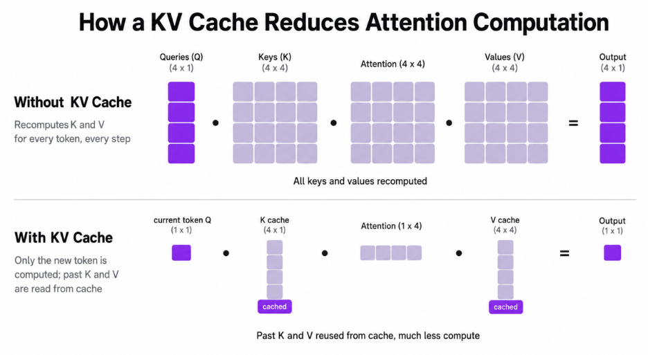
LLMs generate text autoregressively: one token at a time, where each new token attends to every token before it. The attention mechanism turns each token into a key and a value vector. Naively, generating token number 1,000 would require recomputing the keys and values for all 999 previous tokens, every single step. That is enormous, redundant work.

The KV cache is the fix: because past tokens never change, their key and value vectors are computed once, stored, and then simply read back on every subsequent step. As NVIDIA puts it in their recent KV cache write-up, this trades a compute bottleneck for a memory one; those K/V tensors now must live somewhere, and they have to be read on every decode step.

That memory cost is not small, and, crucially, it grows linearly with both context length and batch size. The size of the KV cache is:

kv_cache_bytes = batch x seq_len x num_layers x num_kv_heads x head_dim x 2 x bytes_per_element

The x 2 is for storing both keys and values. Plugging in the published config for Llama-3.1-70B (80 layers, 8 KV heads, head dimension 128), the per-token cost and totals work out to:

Read the last row: in FP16, a single 128K-token request needs 40 GiB of KV cache, half of an 80 GB NVIDIA H100, before you have served anyone else. This is why long-context and high-concurrency serving live or die on KV cache efficiency, and why every technique below ultimately buys you one of two things: more effective tokens per gigabyte, or fewer gigabytes per token.

How The Cache Behaves Inside a Server

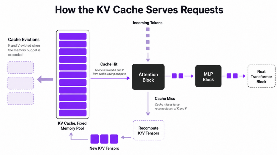
During inference, the cache is filled and used across two phases. In the prefill phase, the model ingests the whole prompt in one big parallel pass and writes K/V for every input token into the cache. In the decode phase it generates tokens one by one; each step reads all cached K/V, computes the new token K/V, and appends it back.

In a real server, the cache is a fixed-size memory pool. When it fills up, the cache manager evicts older entries. If a later request needs an evicted span, you take a cache miss and must recompute it, exactly the work the cache was meant to avoid. As NVIDIA notes, the real-world payoff therefore hinges on cache-hit rate: high hit rates preserve the compute savings; low hit rates push you back toward recomputation.

The Optimisation Landscape

The most useful map of this space is the survey A Survey on Large Language Model Acceleration based on KV Cache Management (Li et al., TMLR 2025). It organises techniques into three levels, and we will use the same structure:

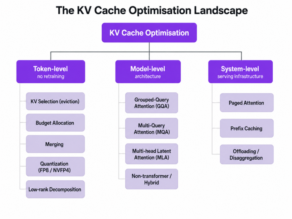
A practical rule of thumb before we dive in: system-level and token-level techniques are things you can turn on without touching the model, so they are where most teams should start. Model-level techniques are decided when you choose a model. Now let's go through each level.

Token-level Optimisation

These techniques operate on the cache itself, leaving the model weights untouched.

KV Cache Selection (Eviction)

Not every token matters equally for future predictions, so one family simply keeps the important K/V entries and drops the rest. The survey splits this into three styles:

• Static selection keeps a fixed pattern of tokens. SnapKV (NeurIPS 2024) and Model Tells You What to Discard / FastGen (ICLR 2024) compress the prompt's KV before generation begins.
• Dynamic selection with permanent eviction drops tokens permanently as it goes. H2O (NeurIPS 2023) keeps a small set of "heavy hitter" tokens that dominate attention; Scissorhands (NeurIPS 2023) exploits the persistence of important tokens; StreamingLLM-style approaches keep a few initial "sink" tokens plus a recent window.
• Dynamic selection without permanent eviction keeps everything but only loads the relevant entries per step. Quest (ICML 2024) and InfLLM (2024) retrieve the most relevant blocks for the current query, so nothing is lost but only a fraction is read.

The trade-off is uniform: eviction saves memory and bandwidth, but risks dropping something a later token needed, which is why "without permanent eviction" approaches have become popular for long-context retrieval workloads.

KV Cache Budget Allocation

Rather than a single global policy, these methods spend a memory budget unevenly where it matters. PyramidKV and PyramidInfer (2024) give earlier layers more cache and later layers less, following the way information funnels through the network. Ada-KV, DuoAttention, and RazorAttention (2024) allocate per attention head, keeping full cache only for the heads that need long-range information (e.g. "retrieval heads") and shrinking the rest.

KV Cache Merging

Instead of discarding tokens, merge similar ones. Intra-layer methods (e.g. CaM, D2O, 2024) merge redundant K/V within a layer; cross-layer methods (MiniCache, KVSharer, 2024) exploit the high similarity of caches between adjacent layers to store one shared copy.

KV Cache Quantisation, The Highest-leverage Practical Lever

Quantisation stores the K/V tensors in fewer bits. It is the most widely deployed token-level technique because it is nearly free to turn on and the accuracy cost is small. The survey groups it into fixed-precision (FlexGen, ZeroQuant), mixed-precision (KIVI, a tuning-free 2-bit scheme; KVQuant, aimed at 10M-token contexts), and outlier-redistribution methods (QuaRot, SmoothQuant, AWQ) that move the hard-to-quantise outliers before quantising.

In production today the practical options are FP8 and, on the newest hardware, NVFP4.

FP8 KV cache (works on NVIDIA H100 today). vLLM supports FP8 KV cache out of the box. Per the vLLM documentation, it roughly doubles the number of tokens you can store, which directly enables longer contexts or higher concurrency. The catch, as the docs state plainly, is that historically FP8 KV cache improved throughput/capacity but not latency, because dequantisation and attention were not fused, although with the FlashAttention-3 backend, attention can now run in the FP8 domain too. Enabling it is one flag:

# vLLM: enable FP8 KV cache when launching the server.
# fp8 == fp8_e4m3 (higher precision); fp8_e5m2 is also available.
vllm serve meta-llama/Llama-3.1-70B-Instruct \
  --tensor-parallel-size 2 \
  --kv-cache-dtype fp8 \        # store K/V in 8-bit instead of 16-bit
  --calculate-kv-scales \       # estimate quant scales dynamically at runtime
  --max-model-len 8192

# The same thing from Python (offline inference).
from vllm import LLM, SamplingParams

llm = LLM(
    model="meta-llama/Llama-3.1-70B-Instruct",
    tensor_parallel_size=2,
    kv_cache_dtype="fp8",        # 8-bit K/V cache
    calculate_kv_scales=True,    # dynamic scale estimation (no calibration step)
)
out = llm.generate("London is the capital of", SamplingParams(temperature=0.7))
print(out[0].outputs[0].text)

For the best accuracy, the vLLM documentation recommends calibrating the quantisation scales against representative data with LLM Compressor rather than estimating them dynamically. One operational note from the field: FP8 and prefix caching interact at the block level. If you toggle kv_cache_dtype between runs, previously cached BF16 blocks won't match new FP8 blocks, so expect a cold cache after switching.

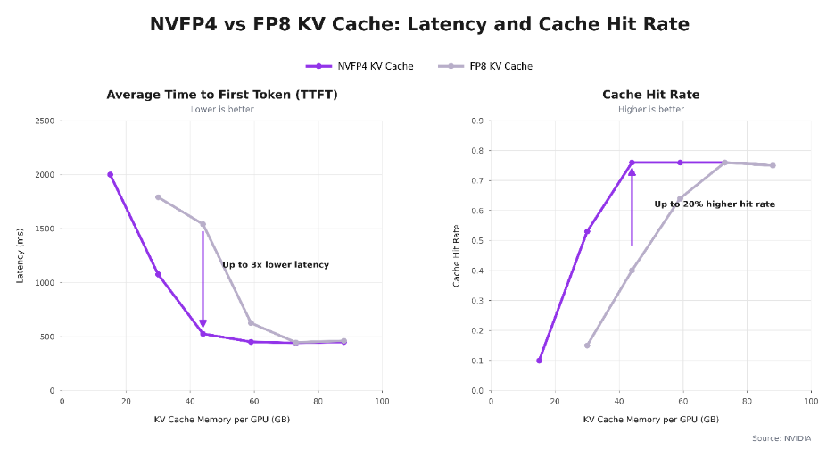
NVFP4 KV cache (NVIDIA Blackwell-generation GPUs). The newest step is NVIDIA's NVFP4, which stores the cache at 4-bit. According to NVIDIA's December 2025 write-up, NVFP4 cuts KV cache footprint by up to ~50% versus FP8 (and therefore ~4x versus FP16), effectively doubling the context budget again, with less than 1% accuracy loss across code-generation, knowledge, and long-context benchmarks (LiveCodeBench, MMLU-PRO, MBPP, Ruler 64K). Mechanically, the current implementation stores K/V in NVFP4 and dequantises to FP8 just before the attention math, so the win comes from fitting far more context on-device, which raises cache-hit rates and cuts prefill recomputation.

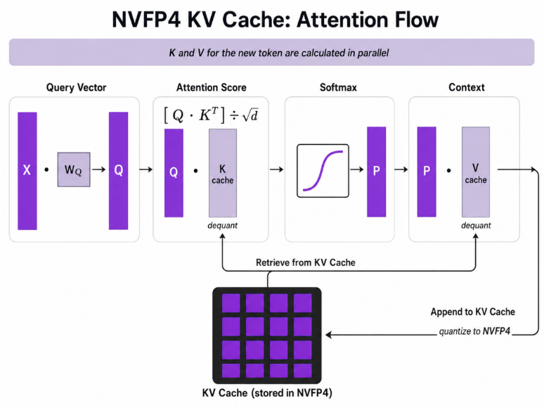
NVIDIA reports that, by holding roughly 2x more context on-device, NVFP4 delivers up to 3x lower time-to-first-token and up to 20% higher cache-hit rates than FP8 as KV-cache memory per GPU grows (measured on Qwen3-Coder-480B-A35B). The gap narrows once the cache is large enough to hold most context. The benefit is biggest exactly when memory is tight.

You produce an NVFP4 KV cache with NVIDIA TensorRT Model Optimiser (post-training quantisation), then serve it with TensorRT-LLM. The configuration is a small change on top of an FP8 setup:

# NVIDIA TensorRT Model Optimizer: FP8 weights/activations + NVFP4 KV cache.
# (Source: NVIDIA NVFP4 KV cache blog, Dec 2025.)
import modelopt.torch.quantisation as mtq

# Start from the FP8 config, then layer NVFP4 KV-cache settings on top.
quant_cfg = mtq.FP8_DEFAULT_CFG
quant_cfg["quant_cfg"].update(mtq.NVFP4_KV_CFG["quant_cfg"])
# (To also get 4-bit weight math, use mtq.NVFP4_DEFAULT_CFG as the base instead.)

def forward_loop(model):              # calibration pass over a small dataset
    for data in calib_set:
        model(data)

model = mtq.quantize(model, quant_cfg, forward_loop)   # PTQ; QAT also supported

# Serve the quantized checkpoint with TensorRT-LLM.
# (Source: TensorRT-LLM quantisation docs.)
from tensorrt_llm import LLM
from tensorrt_llm.llmapi import KvCacheConfig

llm = LLM(model="/path/to/nvfp4-checkpoint",
          kv_cache_config=KvCacheConfig(dtype="nvfp4"))   # or dtype="fp8"
llm.generate("Hello, my name is")

KV Cache Low-rank Decomposition

The last token-level family compresses K/V along their hidden dimension using low-rank structure. Palu, Eigen Attention, and ShadowKV (2024) project keys and values into a smaller subspace (often via SVD) and reconstruct them on the fly, trading a little compute for a smaller cache.

Model-level Optimisation

These techniques change the architecture that produces the cache. You generally get them by choosing the right model rather than by flipping a serving flag, but they are the most powerful, because they shrink the cache at the source.

Attention Grouping and Sharing: MQA → GQA → Cross-layer

Standard Multi-Head Attention (MHA) stores a separate K/V for every attention head, the most expensive option. Two now-standard ideas reduce this:

Multi-Query Attention (MQA) (Shazeer, 2019) shares a single K/V head across all query heads, maximal saving, some quality loss. Grouped-Query Attention (GQA) (Ainslie et al., EMNLP 2023) is the middle ground used by Llama 3, Qwen, and most modern models: query heads are split into a few groups that each share one K/V head.

This is not a minor effect. Our calculator shows it directly: a hypothetical 70B with full MHA (64 K/V heads) would need 2,560 KiB per token, whereas the real Llama-3.1-70B with GQA (8 K/V heads) needs 320 KiB per token, an 8x reduction, exactly the group ratio, just from the attention design. Cross-layer sharing methods (e.g. CLA, MLKV, 2024) push further by sharing K/V across layers.

Multi-head Latent Attention (MLA): The Architectural Endgame

DeepSeek's Multi-head Latent Attention (MLA), introduced in DeepSeek-V2 (2024) and carried through V3/R1, compresses keys and values into a shared low-rank latent vector, which is what gets cached, then up-projects it during attention. It reduces the cache far more than GQA while, per DeepSeek, matching or beating MHA on quality.

Because most existing open models are GQA, there is active work on converting them to MLA without pretraining from scratch: MHA2MLA (2025) reports reducing Llama-2-7B's KV cache by 92.19% with only a 0.5% LongBench drop using 3 to 6% of the data, and TransMLA (2025) reports 93% KV-cache compression on Llama-2-7B with a 10.6x speedup at 8K context after fine-tuning on ~6B tokens. The takeaway for practitioners: if KV memory dominates your costs and you can adopt a DeepSeek-style model, MLA is the most aggressive lever available.

Non-transformer and Hybrid Architectures

A more radical option is to reduce reliance on attention entirely. State-space and recurrent models such as Mamba and RWKV, and hybrids like Jamba-style designs, maintain a fixed-size recurrent state instead of an ever-growing KV cache, eliminating the linear-growth problem, at the cost of different quality and ecosystem trade-offs.

System-level Optimisation

These are the serving-infrastructure techniques, and the good news is they are the easiest to adopt because they need no model changes. They are also where serving engines like vLLM do much of their work.

PagedAttention: Stop Wasting Memory to Fragmentation

Before PagedAttention (Kwon et al., SOSP 2023, the paper that launched vLLM), serving engines reserved a contiguous chunk of memory for each sequence's maximum possible length, wasting most of it. PagedAttention treats KV memory like an operating system's virtual memory: it splits the cache into fixed-size blocks, allocates them on demand, and indirects through a block table. The result is near-zero fragmentation and the ability to pack many more sequences into the same NVIDIA GPU, the foundation that makes most of the other system-level wins possible. With vLLM you get it automatically.

Prefix Caching: Reuse Work Across Requests

If many requests share a prefix (a long system prompt, a few-shot template, a document being asked about repeatedly), you should compute that prefix's KV once and reuse it. vLLM's Automatic Prefix Caching (enabled by default in vLLM V1) hashes prompt blocks and reuses any whose hash it has already seen; SGLang's RadixAttention does the same with a radix tree. For agent loops, multi-tenant SaaS, and document Q&A, this is often the single highest-impact optimisation because a cache hit skips prefill entirely.

# Prefix caching is on by default in vLLM V1. To control it explicitly:
vllm serve meta-llama/Llama-3.1-70B-Instruct \
  --tensor-parallel-size 2 \
  --enable-prefix-caching        # (use --no-enable-prefix-caching to disable)

In shared/multi-tenant environments, vLLM also supports per-request cache_salt so that cached blocks are only reused by requests with the same salt, preventing one tenant from inferring another's cached content from latency.

Offloading And Disaggregation: Spend Cheaper Memory

When NVIDIA GPU memory genuinely runs out, you can spill the KV cache to CPU RAM (and research systems like FlexGen and InstInfer go as far as SSD) or run prefill and decode on separate pools (disaggregation, e.g. DistServe, OSDI 2024). Offloading trades PCIe/host bandwidth for capacity. In vLLM it is a single argument:

# Offload up to 10 GiB of KV cache per NVIDIA GPU to CPU RAM, a "virtual" memory bump.
vllm serve meta-llama/Llama-3.1-70B-Instruct \
  --tensor-parallel-size 2 \
  --cpu-offload-gb 10

How to Put It Together: Quick Steps

You rarely pick one technique; they stack. A sensible order of operations when you are KV-memory bound on Hyperstack NVIDIA GPUs:

1. Turn on the free system-level wins first. PagedAttention is automatic in vLLM; enable prefix caching (default in V1); for workloads with shared prefixes, this alone can be the biggest single improvement.
2. Quantise the cache. On NVIDIA H100 (NVIDIA Hopper) VMs, add --kv-cache-dtype fp8 for roughly 2x the KV capacity at minimal accuracy cost; calibrate scales with LLM Compressor for production. On NVIDIA Blackwell-generation hardware, NVFP4 roughly doubles capacity again.
3. Choose the right architecture. When selecting a model, prefer GQA (Llama 3, Qwen) over MHA, and consider MLA (DeepSeek-style) if KV memory dominates your cost and you need a very long context.
4. Apply token-level eviction/selection (e.g. SnapKV-style compression, or Quest-style retrieval) if a specific long-context workload still doesn't fit.
5. Offload to CPU with --cpu-offload-gb only as a last resort; it buys capacity at the cost of bandwidth.

A reasonable starting point for a long-context, high-concurrency 70B deployment on a 2x NVIDIA H100 GPU VM:

vllm serve meta-llama/Llama-3.1-70B-Instruct \
  --tensor-parallel-size 2 \        # shard the model across 2 NVIDIA GPUs
  --kv-cache-dtype fp8 \            # ~2x KV capacity on NVIDIA Hopper
  --calculate-kv-scales \           # dynamic scales (swap for LLM Compressor in prod)
  --enable-prefix-caching \         # reuse shared system prompts / documents
  --gpu-memory-utilization 0.90 \   # give the KV cache as much room as is safe
  --max-model-len 32768             # context length you intend to support

To see the effect, measure before and after with vLLM's built-in load generator and watch the reported KV-cache blocks rise when you enable FP8:

vllm bench serve \
  --model meta-llama/Llama-3.1-70B-Instruct \
  --dataset-name random --random-input-len 4096 --random-output-len 256 \
  --num-prompts 1000 --max-concurrency 128

Conclusion

The KV cache is where LLM inference economics are won or lost. The good news is that the cheapest wins are also the easiest: PagedAttention and prefix caching come essentially for free in vLLM, and FP8 KV cache is a single flag that roughly doubles your capacity. From there, NVFP4 on NVIDIA Blackwell, GQA/MLA architectures, and token-level eviction give you progressively more headroom for the longest contexts and the largest batches. Stacked together, these techniques are the difference between a context length you can't afford and one you can serve profitably.

Optimise Your LLM Serving Stack

KV cache efficiency can be the difference between serving long-context workloads profitably and running into GPU memory limits long before your infrastructure is fully utilised.

If you're deploying on NVIDIA H100 today or planning for future capacity, Hyperstack provides the GPU infrastructure needed to scale inference with support for modern serving frameworks, long-context deployments and high-concurrency workloads.

Teams with regulated, sensitive or sovereignty requirements can also reserve NVIDIA Blackwell and NVIDIA Blackwell Ultra clusters through Hyperstack Secure Private Cloud, giving them dedicated AI infrastructure within a single-tenant environment.

Ready to improve throughput, reduce memory overhead and lower cost per token? Get started on Hyperstack.

 

FAQs